MLPR → Course Notes → w8c
PDF of this page
Previous: Netflix Prize
Next: Computing logistic regression predictions
$$\notag
\newcommand{\D}{\mathcal{D}}
\newcommand{\M}{\mathcal{M}}
\newcommand{\N}{\mathcal{N}}
\DeclareMathOperator*{\argmax}{arg\,max}
\DeclareMathOperator*{\argmin}{arg\,min}
\newcommand{\bdelta}{{\boldsymbol{\delta}}}
\newcommand{\be}{\mathbf{e}}
\newcommand{\bm}{\mathbf{m}}
\newcommand{\bmu}{{\boldsymbol{\mu}}}
\newcommand{\bw}{\mathbf{w}}
\newcommand{\bx}{\mathbf{x}}
\newcommand{\by}{\mathbf{y}}
\newcommand{\eye}{\mathbb{I}}
\newcommand{\g}{\,|\,}
\newcommand{\intd}{\;\mathrm{d}}
\newcommand{\la}{\!\leftarrow\!}
\newcommand{\nth}{^{(n)}}
\newcommand{\pdd}[2]{\frac{\partial #1}{\partial #2}}
\newcommand{\te}{\!=\!}
\newcommand{\tm}{\!-\!}
\newcommand{\tp}{\!+\!}
$$
Bayesian logistic regression and Laplace approximations
So far we have only performed probabilistic inference in two particularly tractable situations: 1) small discrete models: inferring the class in a Bayes classifier, the card game, the robust logistic regression model. 2) “linear-Gaussian models”, where the observations are linear combinations of variables with Gaussian beliefs, to which we add Gaussian noise.
For most models, we cannot compute the equations for making Bayesian predictions exactly. Logistic regression will be our working example. We’ll look at how Bayesian predictions differ from regularized maximum likelihood. Then we’ll look at different ways to approximately compute the integrals.
As a quick review, the logistic regression model gives the probability of a binary label given a feature vector: \[
P(y\te1\g\bx, \bw) \,=\, \sigma(\bw^\top\bx) \,=\, 1/(1+e^{-\bw^\top\bx}).
\] We usually add a bias parameter \(b\) to the model, making the probability \(\sigma(\bw^\top\bx\tp b)\). Although the bias is often dropped from the presentation, to reduce clutter. We can always work out how to add a bias back in, by including a constant element in the input features \(\bx\).
You’ll see various notations used for the training data \(\D\). The model gives the probability of a vector of outcomes \(\by\) associated with a matrix of inputs \(X\) (where the \(n\)th row is \(\bx^{(n)\top}\)). Maximum likelihood fitting maximizes the probability: \[
P(\by\g X, \bw) = \prod_n \sigma(z\nth \bw^\top\bx\nth), \qquad \text{where}~z\nth = 2y\nth \tm 1,~~\text{if}~~ y\nth \in \{0,1\}.
\] For compactness, we’ll write this likelihood as \(P(\D\g\bw)\), even though really only the outputs \(\by\) in the data are modelled. The inputs \(X\) are assumed fixed and known.
Logistic regression is most frequently fitted by a regularized form of maximum likelihood. For example L2 regularization fits an estimate \[
\bw^* = \argmax_\bw \left[\log P(\by\g X, \bw) - \lambda \bw^\top\bw\right].
\] We find a setting of the weights that make the training data appear probable, but discourage fitting extreme settings of the weights, that don’t seem reasonable. Usually the bias weight will be omitted from the regularization term.
Just as with simple linear regression, we can instead follow a Bayesian approach. The weights are unknown, so predictions are made considering all possible settings, weighted by how plausible they are given the training data.
The posterior distribution over the weights is given by Bayes’ rule: \[
p(\bw\g\D) = \frac{P(\D\g\bw)\,p(\bw)}{P(\D)}
\propto P(\D\g\bw)\,p(\bw).
\] The normalizing constant is the integral required to make the posterior distribution integrate to one: \[
P(\D) = \int P(\D\g\bw)\,p(\bw)\intd\bw.
\]
The figures below are for five different plausible sets of parameters, sampled from the posterior \(p(\bw\g\D)\). Each figure shows the decision boundary \(\sigma(\bw^\top\bx)\te0.5\) for one parameter vector as a solid line, and two other contours given by \(\bw^\top\bx\te\pm1\).

The axes in the figures above are the two input features \(x_1\) and \(x_2\). The model included a bias parameter, and the model parameters were sampled from the posterior distribution given data from the two classes as illustrated. The arrow, perpendicular to the decision boundary, illustrates the direction and magnitude of the weight vector.
Assuming that the data are well-modelled by logistic regression, it’s clear that we don’t know what the correct parameters are. That is, we don’t know what parameters we would fit after seeing substantially more data. The predictions given the different plausible weight vectors differ substantially.
The Bayesian way to proceed is to use probability theory to derive an expression for the prediction we want to make: \[\begin{align}
P(y\g \bx, \D) &= \int p(y,\bw\g \bx, \D)\intd\bw\\
&= \int P(y\g \bx,\bw)\,p(\bw\g\D)\intd\bw.
\end{align}\] That is, we should average the predictive distributions \(P(y\g\bx,\bw)\) for different parameters, weighted by how plausible those parameters are, \(p(\bw\g\D)\). Contours of this predictive distribution, \(P(y\te1\g\bx,\D) \in \{0.5, 0.27, 0.73, 0.12,0.88\}\), are illustrated in the left panel below. Predictions at some constant distance away from the decision boundary are less certain when further away from the training inputs. That’s because the different predictors above disagreed in regions far from the data.

Again, the axes are the input features \(x_1\) and \(x_2\). The right hand figure shows \(P(y\te1\g \bx,\bw^*)\) for some fitted weights \(\bw^*\). No matter how these fitted weights are chosen, the contours have to be linear. The parallel contours mean that the uncertainty of predictions falls at the same rate when moving away from the decision boundary, no matter how far we are from the training inputs.
It’s common to describe L2 regularized logistic regression as MAP (Maximum a posteriori) estimation with a Gaussian \(\N(0,\sigma_w^2\eye)\) prior on the weights. The “most probable” weights, coincide with an L2 regularized estimate: \[
\bw^* = \argmax_\bw \left[\log p(\bw\g \D)\right] =
\argmax_\bw \left[ \log P(\D\g \bw) - \frac{1}{2\sigma_w^2}\bw^\top\bw \right].
\] MAP estimation is not a “Bayesian” procedure. The rules of probability theory don’t tell us to fix an unknown parameter vector to an estimate. We could view MAP as an approximation to the Bayesian procedure, but the figure above illustrates that it is a crude one: the Bayesian predictions (left) are qualitatively different to the MAP ones (right).
Unfortunately, we can’t evaluate the integral for predictions \(P(y\g\bx,\D)\) in closed form. Making model choices for Bayesian logistic regression is also computationally challenging. The marginal probability of the data, \(P(\D)\), is the marginal likelihood of the model, which we might write as \(P(\D\g\M)\) when we are evaluating some model choices \(\M\) (such as basis functions and hyperparameters). We also can’t evaluate the integral for \(P(\D)\) in closed form.
We’re able to do some integrals involving Gaussian distributions. The posterior distribution over the weights \(p(\bw\g\D)\) is not Gaussian, but we can make progress if we can approximate it with a Gaussian.
First, I’ve contrived an example to illustrate how the posterior over the weights can look non-Gaussian. We have a Gaussian prior with one sigmoidal likelihood term. Here we assume we know the bias is 10, and we have one datapoint with \(y\te1\) at \(x\te-20\): \[
\begin{align}
p(w) \,&\propto\, \N(w; 0, 1)\\
p(w\g \D) \,&\propto\, \N(w; 0, 1)\,\sigma(10 - 20w).
\end{align}
\] We are now fairly sure that the weight isn’t a large positive value, because otherwise we’d have probably seen \(y\te0\). We (softly) slice off the positive region and renormalize to get the posterior distribution illustrated below:
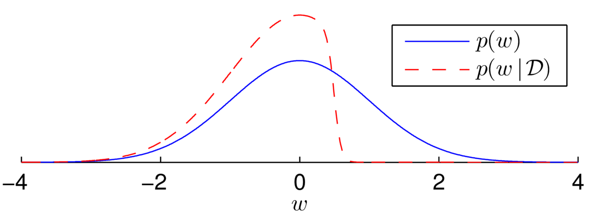
The distribution is asymmetric and so clearly not Gaussian. Every time we multiply the posterior by a sigmoidal likelihood, we softly carve away half of the weight space in some direction. While the posterior distribution has no neat analytical form, the distribution over plausible weights often does look Gaussian after many observations.
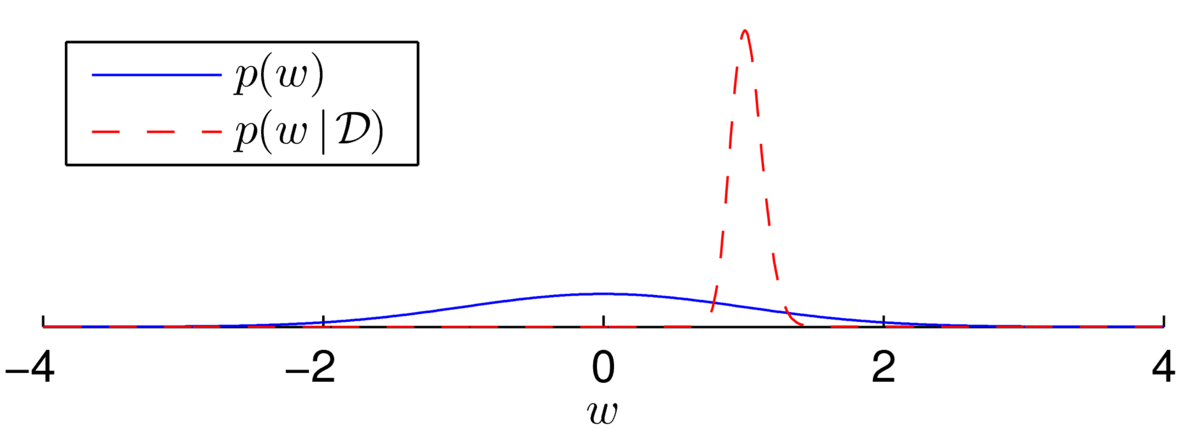
As another example, I generated \(N\te500\) labels, \(\{z\nth\}\), from a logistic regression model with no bias and with \(w\te1\) at \(x^{(n)}\sim \N(0,10^2)\). Then, \[
\begin{align}
p(w) \,&\propto\, \N(w; 0, 1)\\
p(w\g \D) \,&\propto\, \N(w; 0, 1)\,\prod_{n=1}^{500}\sigma(wx^{(n)}z^{(n)}), \qquad z\nth \in \{\pm1\}.
\end{align}
\] The posterior now appears to be a beautiful bell-shape:
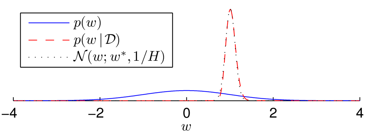
Fitting a Gaussian distribution (using the Laplace approximation, next section) shows that the distribution isn’t quite Gaussian… but it’s close:
There are multiple ways that we could try to fit a distribution with a Gaussian form. For example, we could try to match the mean and variance of the distribution. The Laplace approximation is another possible way to approximate a distribution with a Gaussian. It can be seen as an incremental improvement of the MAP approximation to Bayesian inference, and only requires some additional derivative computations.
We can only evaluate the posterior distribution up to a constant: we can evaluate the joint probability \(p(\bw,\D)\), but not the normalizer \(P(\D)\). We match the shape of the posterior using \(p(\bw,\D)\), and then the approximation can be used to approximate \(P(\D)\).
The Laplace approximation sets the mode of the Gaussian approximation to the mode of the posterior distribution, and matches the curvature of the log probability density at that location. We need to be able to evaluate first and second derivatives of \(\log P(\bw,\D)\).
The rest of the notes just fills in the details. I’m not adding much to MacKay’s textbook pp341–342, or Murphy’s book p255. Although I try to go slightly more slowly and show some pictures of what can go wrong. A concrete example is given by one of MacKay’s questions reproduced at the bottom of this note. A worked answer is given in the next note.
First of all we find the most probable setting of the parameters: \[
\bw^* = \argmax_\bw\, p(\bw\g\D) = \argmax_\bw\, \log p(\bw,\D).
\] The conditional probability on the left is what we intuitively want to optimize. The maximization on the right gives the same answer, but contains the term we will actually compute. Reminder: why do we take the log?
We usually find the mode of the distribution by minimizing an ‘energy’, which is the negative log-probability of the distribution up to a constant. For a posterior distribution, we can define the energy as: \[
E(\bw) = - \log p(\bw,\D), \qquad \bw^* = \argmin_\bw E(\bw).
\] We minimize it as usual, using a gradient-based numerical optimizer.
The minimum of the energy is a turning point. For a scalar variable \(w\) the first derivative \(\pdd{E}{w}\) is zero and the second derivative gives the curvature of this turning point: \[
H = \left. \frac{\partial^2 E(w)}{\partial w^2} \right|_{w=w^*}.
\] The notation means that we evaluate the second derivative at the optimum, \(w=w^*\). If \(H\) is large, the slope (the first derivative) changes rapidly from a steep descent to a steep ascent. We should approximate the distribution with a narrow Gaussian. Generalizing to multiple variables \(\bw\), we know \(\nabla_\bw E\) is zero at the optimum and we evaluate the Hessian, a matrix with elements: \[
H_{ij} = \left. \frac{\partial^2 E(\bw)}{\partial w_i\partial w_j} \right|_{\bw=\bw^*}.
\] This matrix tells us how sharply the distribution is peaked in different directions.
For comparison, we can find the optimum and curvature that we would get if our distribution were Gaussian. For a one-dimensional distribution, \(\N(\mu, \sigma^2)\), the energy (the negative log-probability up to a constant) is: \[
E_\N(w) = \frac{(w-\mu)^2}{2\sigma^2}.
\] The minimum is \(w^*=\mu\), and the second derivative \(H = 1/\sigma^2\), implying the variance is \(\sigma^2 = 1/H\). Generalizing to higher dimensions, for a Gaussian \(\N(\bmu,\Sigma)\), the energy is: \[
E_\N(\bw) = \frac{1}{2} (\bw-\bmu)^\top \Sigma^{-1} (\bw-\bmu),
\] with \(\bw^*=\bmu\) and \(H = \Sigma^{-1}\), implying the covariance is \(\Sigma = H^{-1}\).
Therefore matching the minimum and curvature of the ‘energy’ (negative log-probability) to those of a Gaussian energy gives the Laplace approximation to the posterior distribution: \[
\fbox{$\displaystyle
p(\bw\g\D) \approx \N(\bw;\, \bw^*, H^{-1})
$}
\]
Evaluating our approximation for a \(D\)-dimensional distribution gives: \[
p(\bw\g\D) = \frac{p(\bw,\D)}{P(\D)} \approx \N(\bw;\, \bw^*, H^{-1}) =
\frac{|H|^{1/2}}{(2\pi)^{D/2}} \exp\left( -\frac{1}{2} (\bw-\bw^*)^\top H(\bw-\bw^*)\right).
\] At the mode \(\bw^*\te\bw\), the exponential term disappears and we get: \[
\frac{p(\bw^*,\D)}{P(\D)} \approx \frac{|H|^{1/2}}{(2\pi)^{D/2}}, \qquad \fbox{$\displaystyle P(\D) \approx \frac{p(\bw^*,\D) (2\pi)^{D/2}}{|H|^{1/2}}$}.
\] An equivalent expression is \[\fbox{$P(\D) \approx p(\bw^*,\D)\, |2\pi H^{-1}|^{1/2},$}\] where \(|\cdot|\) means take the determinant of the matrix.
When some people say “the Laplace approximation”, they are referring to this approximation of the normalization \(P(\D)\), rather than the intermediate Gaussian approximation to the distribution.
If we think that the Energy is well-behaved and sharply peaked around the mode of the distribution, we might think that we can approximate it with a Taylor series. In one dimension we write \[
\begin{align}
E(w^* + \delta) &\approx E(w^*) \;+\; \left.\pdd{E}{w}\right|_{w^*}\delta \;+\;
\frac{1}{2}\left.\frac{\partial^2 E}{\partial w^2}\right|_{w^*}\delta^2\\
&\approx E(w^*) \;+\; \frac{1}{2}H\delta^2,
\end{align}
\] where the second term disappears because \(\pdd{E}{w}\) is zero at the optimum. In multiple dimensions this Taylor approximation generalizes to: \[
E(\bw^* + \bdelta) \approx E(\bw^*) + {\textstyle\frac{1}{2}}\bdelta^\top \!H\bdelta.
\] A quadratic energy (negative log-probability) implies a Gaussian distribution. The distribution is close to the Gaussian fit when the Taylor series is accurate.
For models with a fixed number of identifiable parameters, the posterior becomes tightly peaked in the limit of large datasets. Then the Taylor expansion of the log-posterior doesn’t need to be extrapolated far and will be accurate. Search term for more information: “Bayesian central limit theorem”.
Despite the theory above, it is easy for the Laplace approximation to go wrong.
In high dimensions, there are many directions in parameter space where there might only be a small number of informative datapoints. Then the posterior could look like the first asymmetrical example in this note.
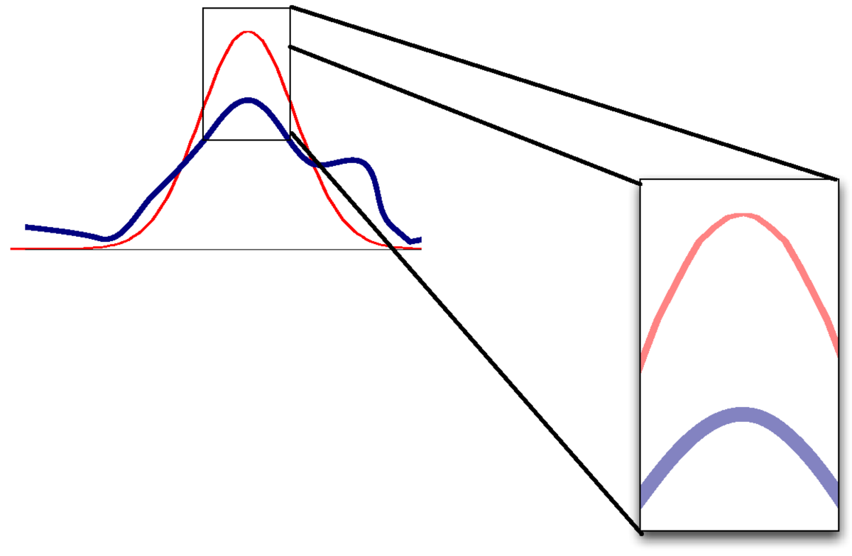
If the mode and curvature are matched, but the distribution is otherwise non-Gaussian, then the value of the densities won’t match.
As a result, the approximation of \(P(\D)\) will be poor.
One way for a distribution to be non-Gaussian is to be multi-modal. The posterior of logistic regression only has one mode, but the posterior for neural networks will be multimodal. Even if capturing one mode is reasonable, an optimizer could get stuck in bad local optima.
In models with many parameters, the posterior will often be flat in some direction, where parameters trade off each other to give similar predictions. When there is zero curvature in some direction, the Hessian isn’t positive definite and we can’t get a meaningful approximation.
Bishop covers the Laplace approximation and application to Bayesian logistic regression in Sections 4.4 and 4.5.
Or read Murphy Sections 8.4 to 8.4.4 inclusive. You can skip 8.4.2 on BIC.
Similar material is covered by MacKay, Ch. 41, pp492–503, and Ch. 27, pp341–342. (Section 41.4 uses non-examinable methods — skim over on first reading.)
The Laplace approximation was used in some of the earliest Bayesian neural networks although — as presented here — it’s now rarely used. However, the idea does occur in recent work, such as on continual learning (Kirkpatrick et al., Google Deepmind, 2017) and a more sophisticated variant is used by the popular statistical package, R-INLA.
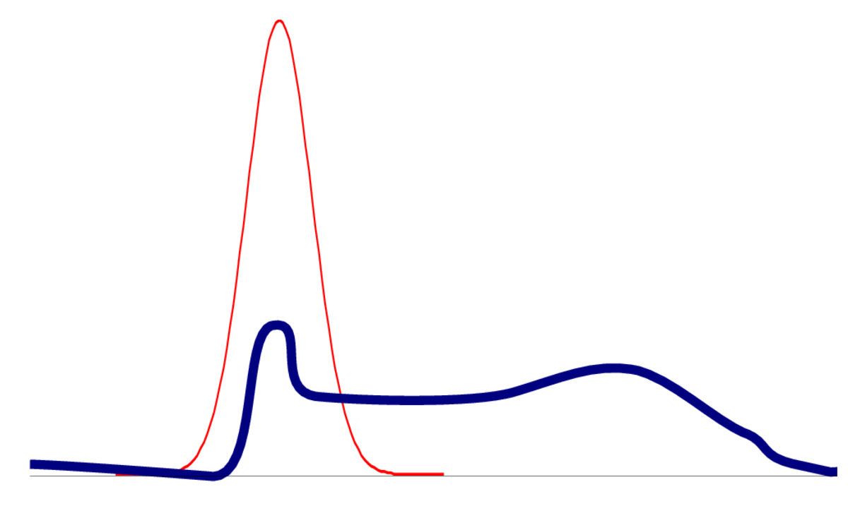
Exercise 27.1 in MacKay’s textbook (p342) is about inferring the parameter \(\lambda\) of a Poisson distribution based on an observed count \(r\). The likelihood function and prior distribution for the parameter are: \[
P(r\g \lambda) = \exp(-\lambda)\frac{\lambda^r}{r!}, \qquad p(\lambda) \propto \frac{1}{\lambda}.
\] Find the Laplace approximation to the posterior over \(\lambda\) given an observed count \(r\).
Now reparameterize the model in terms of \(\ell\te\log\lambda\). After performing the change of variables, the improper prior on \(\log\lambda\) becomes uniform, that is \(p(\ell)\) is constant. Find the Laplace approximation to the posterior over \(\ell\te\log\lambda\).
Which version of the Laplace approximation is better? It may help to plot the true and approximate posteriors of \(\lambda\) and \(\ell\) for different values of the integer count \(r\).
MLPR → Course Notes → w8c
PDF of this page
Previous: Netflix Prize
Next: Computing logistic regression predictions
Notes by Iain Murray and Arno Onken