MLPR → Course Notes → w1c
PDF of this page
Previous: Linear regression
Next: Training, Testing, and Evaluating Different Models
$$\notag
\newcommand{\I}{\mathbb{I}}
\newcommand{\N}{\mathcal{N}}
\newcommand{\bw}{\mathbf{w}}
\newcommand{\bx}{\mathbf{x}}
\newcommand{\by}{\mathbf{y}}
\newcommand{\la}{\!\leftarrow\!}
\newcommand{\noo}[1]{\frac{1}{#1}}
\newcommand{\nth}{^{(n)}}
\newcommand{\ra}{\!\rightarrow\!}
\newcommand{\te}{\!=\!}
\newcommand{\tm}{\!-\!}
\newcommand{\ttimes}{\!\times\!}
$$
Linear regression, overfitting, and regularization
The fitted function \(f(\bx)\) doesn’t usually match the training data exactly. Each training item has a residual, \((y\nth \tm f(\bx\nth))\), which is normally non-zero. Why don’t we get perfect fits?
Data is usually inherently noisy or stochastic, in which case it’s impossible to exactly predict \(y\) from \(\bx\). For example, if a builder mixes several batches of concrete with the same quantities specified by \(\bx\), we wouldn’t expect their observed strengths \(y\) to be exactly the same.
Even if the outputs are noiseless, \(N\!>\!D\) data-points are unlikely to lie exactly on any function represented by a linear combination of our \(D\) basis functions.
If we don’t include enough basis functions, we will underfit our data. For example, if some points lie exactly along a cubic curve:
N = 100; D = 1;
X = rand(N, D) - 0.5; % np.random.rand in NumPy
yy = X.^3;            % X**3 in NumPy
We would not be able to fit this data accurately if we only put linear and quadratic basis functions in our augmented design matrix \(\Phi\).
You could fit the cubic data above fairly accurately with a few RBF functions. The fit wouldn’t extrapolate well outside the \(x\!\in\!(-0.5,0.5)\) range of observations, but you can get an accurate fit close to where there is data. To avoid underfitting, we need a model with enough representational power to closely approximate the underlying function.
When the number of training points \(N\) is small, it’s easy to fit the observations with low square error. In fact, usually if we have \(N\) or more basis functions, such as \(N\) RBFs with different centres, the residuals will all be zero! However, we should not trust this fit. It’s hard for us as intelligent humans to guess what an arbitrary function is doing in between only a few observations, so we shouldn’t believe the result of fitting an arbitrary model either. Moreover, if the observations are noisy, it seems unlikely that a good fit should match the observed data exactly anyway.
As advocated by Acton in note w1a, one possible approach to modelling is as follows. Start with a simple model with only a few parameters. This model may underfit, that is, not represent all of the structure evident in the training data. We could then consider a series of more complicated models while we feel that fitting these models can still be justified by the amount of data we have.
However, limiting the number of parameters in a model isn’t always easy or the right approach. If our inputs have many features, even simple linear regression (without additional basis functions) has many parameters. An example is predicting some characteristic of an organism (a phenotype) from DNA data, which is often in the form of \(>\!10^5\) features. We could consider doing some preliminary filtering to remove features, although this choice is itself a fit of sorts to the data. Moreover, filtering is not always the correct answer. Perhaps we have features that are noisy measurements of the same underlying property. In that case we should average the measurements rather than selecting one of them. However, we may not know in advance which groups of features should be averaged, and which selected.
Another approach to modelling is to use large models (models with many free parameters), but to disallow unreasonable fits that match our noisy training data too closely.
Example 1: Fitting many features. We will consider a synthetic situation where each datapoint relates to a different underlying quantity \(\mu\nth\). We will sample each of these quantities from a uniform distribution between zero and one, which we write \[
\begin{align}
\mu\nth &\sim \mathrm{Uniform}(0,1).
\end{align}
\] In our example, the features and output will both be noisy measurements of the underlying quantity: \[
\begin{align}
x_d\nth &\sim \N(\mu\nth,0.01^2), \quad d=1\dots D\\
y\nth &\sim \N(\mu\nth,0.1^2).
\end{align}
\] The notation \(\N(\mu,\sigma^2)\) means the values are drawn from a Gaussian or Normal distribution centred on \(\mu\), with variance \(\sigma^2\).
In this situation, averaging the \(x_d\) measurements would be a reasonable estimate of the underlying feature \(\mu\), and hence the output \(y\). Thus a regression model with \(w_d\te \noo{D}\) would make reasonable predictions of \(y\) from \(\bx\). Do you recover something like this model if you fit linear regression? Try fitting randomly-generated datasets with various \(N\) and \(D\). One of the following code snippets may help:
% Matlab, mu is Nx1
X = repmat(mu, 1, D) + 0.01*randn(N, D);
# Python, mu is (N,)
X = np.tile(mu[:,None], (1, D)) + 0.01*np.random.randn(N, D)
By making \(D\) large and \(N\) not much larger than \(D\), the weights that give the best least-squares fit to the training data are much larger in magnitude than \(w_d\te \noo{D}\). By using weights much smaller and larger than the ideal values, the model can use small differences between input features to fit the noise in the observations. If we tried to interpret the value of a weight as meaning something about the corresponding feature, we would embarrass ourselves. However, the average of the weights is often close to \(\noo{D}\), and predictions on more data generated in the same way as above, might be ok. The model will generalize badly though — it will make wild predictions — if we test on inputs generated from \(x_d \sim \N(\mu,1)\).
Example 2: Explaining noise with many basis functions. Consider data drawn as follows: \[
\begin{align}
x_d\nth &\sim \mathrm{Uniform}[0,1], \quad d=1\dots D\\
y\nth &\sim \N(0,1).
\end{align}
\] The outputs have no relationship to the inputs. The predictor with the smallest average square error on future test cases is \(f(\bx)\te0\), its average square error will be one. We now consider what happens if we fit a model with many basis functions. If we use a high-degree polynomial, or many RBF basis functions, we can get a lower square training error than one. However, the error on new data would be larger. The fits usually have extreme weights with large magnitudes (for example \({\sim\!10^3}\)). There is a danger that for some inputs, the predictions could be extreme.
It’s possible to represent a large range of interesting functions using weights with small magnitude. Yet least-square fits are often obtained with combinations of extremely positive and negative weights, obtaining fits that pass unreasonably close to noisy observations. We would like to avoid fitting these extreme weights.
Penalizing extreme solutions can be achieved in various ways, and is called regularization. One form of regularization is to penalize the sum of the square weights in our cost function. This method has various names, including Tikhonov regularization, ridge regression, or \(L_2\) regularization. For \(K\) basis functions, the regularized cost function is then: \[
\begin{align}
E_\lambda(\bw;\,\by,\Phi) &= \sum_{n=1}^N \left[ y\nth - f(\bx\nth; \bw) \right]^2 +
\lambda \sum_{k=1}^K w_k^2\\
&= (\by - \Phi\bw)^\top (\by - \Phi\bw) + \lambda \bw^\top\bw.
\end{align}
\] For \(\lambda\te0\) we only care about fitting the data, but for larger values of \(\lambda\) we trade-off the accuracy of the fit so that we can make the weights smaller in magnitude.
We can fit the regularized cost function with the same linear least-squares fitting routine as before. This time, instead of adding new features, we add new data items. If our original matrix of input features \(\Phi\) is \(N\ttimes K\), for \(N\) data items and \(K\) basis functions, we add \(K\) rows to both the vector of labels and matrix of input features: \[
\tilde{\by} = \left[\begin{array}{c}\by\\ \mathbf{0}_K\end{array}\right]
\quad
\tilde{\Phi} = \left[\begin{array}{c}\Phi\\ \sqrt{\lambda}\I_K\end{array}\right],
\] where \(\mathbf{0}_K\) is a vector of \(K\) zeros, and \(\I_K\) is the \(K\ttimes K\) identity matrix. Then \[
\begin{align}
E(\bw;\,\tilde{\by},\tilde{\Phi}) &= (\tilde{\by} - \tilde{\Phi}\bw)^\top (\tilde{\by} - \tilde{\Phi}\bw)\\
&= (\by - \Phi\bw)^\top (\by - \Phi\bw) + \lambda\bw^\top\bw
= E_\lambda(\bw;\,\by,\Phi).
\end{align}
\] Thus we can fit training data \((\tilde{\by},\tilde{\Phi})\) using least-squares code that knows nothing about regularization, and fit the regularized cost function.
Below we see a situation where using least-squares with a dozen RBF basis functions leads to overfitting.
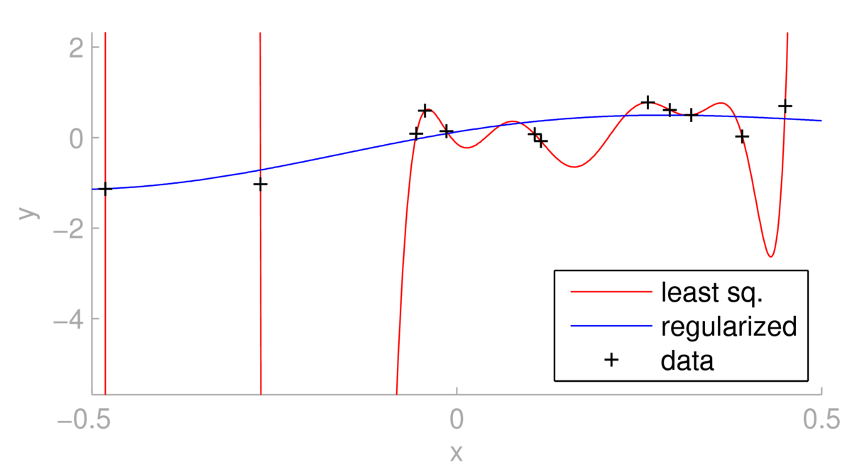
One could argue for changing the basis functions. However, as illustrated above, regularizing the same linear regression model can give less extreme predictions, at the expense of giving a fit further from the training points. The regularized fit depends strongly on \(\lambda\). For \(\lambda\te0\) we obtain the least squares fit. What happens as \(\lambda\ra\infty\)?
Using either Matlab or Python, make sure you can generate some example data, construct a matrix of features \(\Phi\), and fit the regularized least squares linear regression weights. Plot the fitted function.
We minimize the cost function \(E_\lambda(\bw;\,\by,\Phi)\) on the training set with respect to the weights \(\bw\). Why would it be a bad idea to minimize the same cost function as a way to set the regularization constant \(\lambda\)?
If we have \(K\) radial basis functions, give a simple upper bound on the largest function value that could be obtained for a given weight vector \(\bw\). Also give a simple upper bound on the largest derivative (you could consider one dimensional regression). From such bounds we can see that limiting the size of the weights stops the function taking on extreme values, or changing extremely quickly.
MLPR → Course Notes → w1c
PDF of this page
Previous: Linear regression
Next: Training, Testing, and Evaluating Different Models
Notes by Iain Murray and Arno Onken