MLPR → Course Notes → w7c
PDF of this page
Previous: Bayesian model choice
Next: Gaussian Processes and Kernels
$$
\newcommand{\E}{\mathbb{E}}
\newcommand{\N}{\mathcal{N}}
\newcommand{\ba}{\mathbf{a}}
\newcommand{\bb}{\mathbf{b}}
\newcommand{\bff}{\mathbf{f}}
\newcommand{\bg}{\mathbf{g}}
\newcommand{\bk}{\mathbf{k}}
\newcommand{\bx}{\mathbf{x}}
\newcommand{\by}{\mathbf{y}}
\newcommand{\eye}{\mathbb{I}}
\newcommand{\g}{\,|\,}
\newcommand{\ith}{^{(i)}}
\newcommand{\jth}{^{(j)}}
\newcommand{\te}{\!=\!}
\newcommand{\tp}{\!+\!}
\newcommand{\ttimes}{\!\times\!}
$$
Gaussian processes
Gaussian processes (GPs) are distributions over functions from an input \(\bx\), which could be high-dimensional and could be a complex object like a string or graph, to a scalar or 1-dimensional output \(f(\bx)\). We will use a Gaussian process prior over functions in a Bayesian approach to regression. Gaussian processes can also be used as a part of larger models.
Goals: 1) model complex functions: not just straight lines/planes, or a combination of a fixed number of basis functions. 2) Represent our uncertainty about the function, for example with error bars. 3) Do as much of the mathematics as possible analytically.
The value of uncertainty
Using Gaussian processes, like Bayesian linear regression, we can compute our uncertainty about a function given data. Error bars are useful when making decisions, or optimizing expensive functions. Examples of expensive functions include ‘efficacy of a drug’, or ‘efficacy of a training procedure for a large-scale neural network’.
In the cartoon below, a black dashed line shows an estimate of a function, with a gray region indicating uncertainty. The function could be performance of a system as a function of its settings. Often the performance of a system doesn’t vary up and down rapidly as a function of one setting, but in high-dimensions there could easily be multiple modes — different combinations of inputs that work quite well.
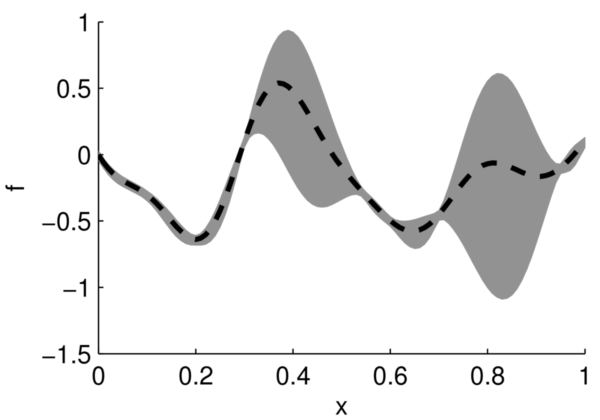
The largest value appears to be around \(x\te0.4\). If we can afford to run a couple of experiments, we might also test the system at \(x\te0.8\), which might actually perform better. According to our point estimates, the performance at \(x\te0\) is similar to \(x\te0.8\). However, we aren’t uncertain at \(x\te0\), so it isn’t worth running experiments there.
Using uncertainty in a probabilistic model to guide search is called Bayesian optimization. We could do Bayesian optimization with Bayesian linear regression. Although we would have to be careful: Bayesian linear regression is often too certain if the model is too simple, or doesn’t include enough basis functions.
Bayesian optimization can also be based on neural networks. However, representing the posterior distribution over parameters, and integrating to give a predictive distribution, is challenging for neural networks.
The multivariate Gaussian distribution
We’ll see that Gaussian processes are really just high-dimensional multivariate Gaussian distributions. This section has a quick review of some of the things we can do with Gaussians. It’s perhaps surprising that these manipulations can answer interesting statistical and machine learning questions!
A Gaussian distribution is completely described by its parameters \(\mu\) and \(\Sigma\): \[
p({\bff}\g \Sigma,\mu) \,=\, \left| 2\pi \Sigma \right|^{-\frac{1}{2}}
\exp\big( -{\textstyle \frac{1}{2}} ({\bff} - \mu)^\top \Sigma^{-1} ({\bff} - \mu) \big),
\] where \(\mu\) and \(\Sigma\) are the mean and covariance: \[
\begin{aligned}
\mu_i &= \E[f_i]\\[0.1in]
\Sigma_{ij} &= \E[f_i f_j] - \mu_i \mu_j.
\end{aligned}
\] The covariance matrix \(\Sigma\) must be positive definite. (Or positive semi-definite if we allow some of the elements of \(\bff\) to depend deterministically on each other.) If we know a distribution is Gaussian and know its mean and covariances, we know its density function.
Any marginal distribution of a Gaussian is also Gaussian. So given a joint distribution: \[
p(\bff,\bg) \,=\, \N\left(
% variable
\left[ \begin{array}{cc}
\bff \\
\bg \\
\end{array}
\right] \!;\;
% mu
\left[ \begin{array}{cc}
\ba \\
\bb \\
\end{array}
\right] \!,\;
% Sigma
\left[ \begin{array}{cc}
A & C \\
C^\top & B \\
\end{array}
\right]
\right),
\] then as soon as you convince yourself that the marginal \[
p(\bff) \,=\, \int p(\bff,\bg)\; \mathrm{d}\bg
\] is Gaussian, you already know the means and covariances: \[
p(\bff) \,=\, \N(\bff;\, \ba, A).
\]
Any conditional distribution of a Gaussian is also Gaussian: \[
p(\bff\g \bg) = \N(\bff;\; \ba \!+\! CB^{-1}(\bg\!-\!\bb),\; A \!-\! CB^{-1}C^\top)
\] Showing this result from scratch requires quite a few lines of linear algebra. However, this is a standard result that is easily looked up (and I wouldn’t make you show it in an exam!).
Representing function values with a Gaussian
We can think of functions as infinite-dimensional vectors. Dealing with the mathematics of infinities and real numbers rigorously is possible but involved. I will side-step these difficulties with a low-tech description.
We could imagine a huge finite discretization of our input space. For example, we could consider only the input vectors \(\bx\) that can be realized with IEEE floating point numbers. After all, those are the only values we’ll ever consider in our code. In theory (but not in practice) we could evaluate a function \(f\) at every discrete location, \(f_i = f(\bx^{(i)})\). If we put all the \(f_i\)’s into a vector \(\bff\), that vector specifies the whole function (up to an arbitrarily fine discretization).
While we can’t store a vector containing the function values for every possible input, it is possible to define a multivariate Gaussian prior on it. Given noisy observations of some of the elements of this vector, it will turn out that we can infer other elements of the vector without explicitly representing the whole object.
If our model is going to be useful, the prior needs to be sensible. If we don’t have any specific domain knowledge, we’ll set the mean vector to zero. If we drew “function vectors” from our prior, an element \(f_i\te f(\bx^{(i)})\), will be positive just as often as it is negative. Defining the covariance is harder. We certainly can’t use a diagonal covariance matrix: if our beliefs about the function values are independent, then observing the function in one location will tell us nothing about its values in other locations. We usually want to model continuous functions: so function values for nearby inputs should have large covariances.
We will define the covariance between two function values using a covariance or kernel function: \[
\mathrm{cov}[f_i, f_j] = k(\bx^{(i)}, \bx^{(j)}).
\] There are families of positive definite kernel functions (“Mercer kernels”), which always produce a positive definite matrix \(K\) if each element is set to \(K_{ij}\te k(\bx^{(i)},\bx^{(j)})\). If the kernel wasn’t positive definite, our prior wouldn’t define a valid Gaussian distribution. One kernel that is positive definite is proportional to a Gaussian: \[
k(\bx^{(i)}, \bx^{(j)}) = \exp(-\|\bx^{(i)}-\bx^{(j)}\|^2),
\] but there are many other choices. For example, another valid kernel is: \[
k(\bx^{(i)}, \bx^{(j)}) = (1 + \|\bx^{(i)}-\bx^{(j)}\|) \exp(-\|\bx^{(i)}-\bx^{(j)}\|).
\] Gaussian processes get their name because they define a Gaussian distribution over a vector of function values. Not because they sometimes use a Gaussian kernel to set the covariances.
Using the Gaussian process for regression
The plot below shows three functions drawn from a Gaussian process prior with zero mean and a Gaussian kernel function.
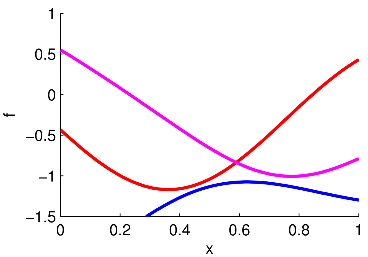
The ‘functions’ plotted here are actually samples from a 100-dimensional Gaussian distribution. Each sample gave the height of a curve at 100 locations along the \(x\)-axis, which were joined up with straight lines. If we chose a different kernel we could get rough functions, straighter functions, or periodic functions.
Our prior is that the function comes from a Gaussian process, \(f\sim\mathcal{GP}\), where a vector of function values has prior \(p(\bff) \te \N(\bff; \mathbf{0}, K)\), where \(f_i = f(\bx^{(i)})\) and \(K_{ij} = k(\bx\ith, \bx\jth)\).
Given noisy observations of some of the function values: \[
y_i \sim \N(f_i, \sigma_y^2),
\] we can update our beliefs about the function. For now we assume the noise variance \(\sigma_y^2\) is fixed and known. According to the model, the observations are centred around one underlying true function as follows:
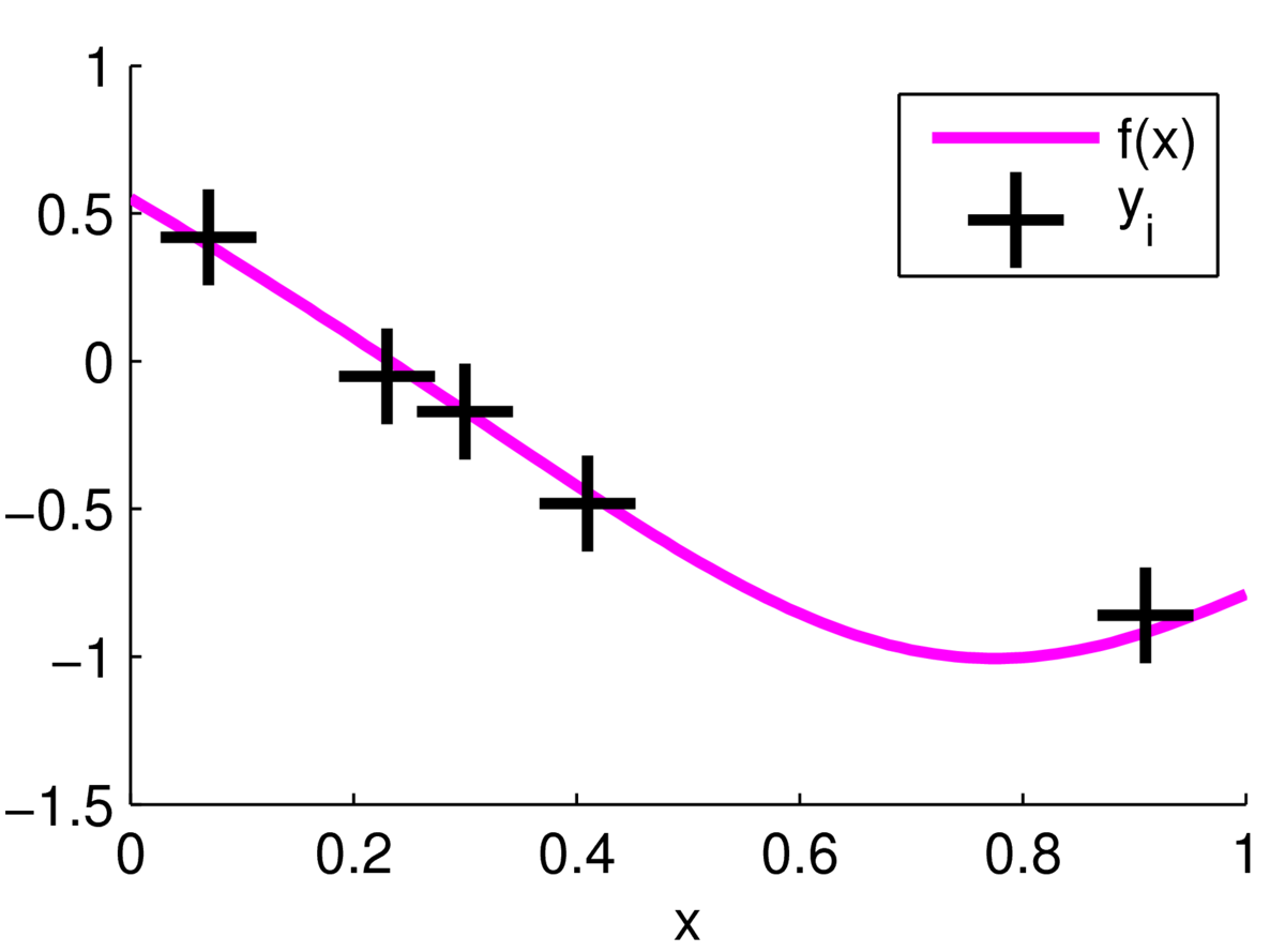
But we don’t know where the function is, we only see the \(\by\) observations.
In 1D we can represent the whole function fairly accurately (as in the plot above) with \({\sim}100\) values. In high-dimensions however, we can’t grid up the input space and explicitly estimate the function everywhere. Instead, we only consider the function at places we have observed, and at test locations \(X_*\te\{\bx^{(*,i)}\}\) where we will make predictions. We call the vector of function values at the test locations \(\bff_*\).
We can write down the model’s joint distribution of the observations and the \(\bff_*\) function values that we’re interested in. This joint distribution is Gaussian, as it’s simply a marginal of our prior over the whole function, with noise added to some of the values: \[
P\left(
\left[ \begin{array}{cc}
\by \\
\bff_* \\
\end{array}
\right] \right) =\, \N\left(
% variables
\left[ \begin{array}{cc}
\by \\
\bff_* \\
\end{array}
\right];\;
% mu
{\bf 0} ,
% Sigma
\left[ \begin{array}{cc}
K(X,X) + \sigma_y^2\eye & K(X,X_*) \\
K(X_*,X) & K(X_*,X_*) \\
\end{array}
\right]
\right),
\] where the compact notation \(K(X, Y)\) follows the Rasmussen and Williams GP textbook (Murphy uses an even more compact notation). Given an \(N\ttimes D\) matrix \(X\) and an \(M\ttimes D\) matrix \(Y\), \(K(X,Y)\) is an \(N\ttimes M\) matrix of kernel values: \[
K(X,Y)_{ij} = k(\bx^{(i)}, \by^{(j)}),
\] where \(\bx^{(i)}\) is the \(i\)th row of \(X\) and \(\by^{(j)}\) is the \(j\)th row of \(Y\).
The covariance of the function values \(\bff_*\) at the test locations, \(K(X_*,X_*)\) is given directly by the prior. The covariance of the observations, \(K(X,X)\tp\sigma_y^2\eye\), is given by the prior, plus the independent noise variance. The cross covariances, \(K(X,X_*)\) come from the prior on functions, the noise has no effect: \[
\begin{aligned}
\mathrm{cov}(y_i, f_{*,j}) &= \E[y_i f_{*,j}] - \E[y_i]\E[f_{*,j}]\\
&= \E[(f_i + \nu_i) f_{*,j}], \quad \nu_i~\text{is noise from}~\N(0,\sigma_y^2),\\
&= \E[f_i f_{*,j}] + \E[\nu_i]\E[f_{*,j}],\\
&= \E[f_i f_{*,j}] = k(\bx^{(i)}, \bx^{(*,j)}).\\
\end{aligned}
\] Because Gaussians marginalize so easily, we can ignore the enormous (or infinite) prior covariance matrix over all of the function values that we’re not interested in.
Using the rule for conditional Gaussians, we can immediately identify that the posterior over function values \(p(\bff_*\g \by)\) is Gaussian with: \[
\begin{aligned}
\text{mean}, \bar{\bff}_* &= K(X_*,X)(K(X,X) + \sigma_y^2\eye)^{-1}\by\\
\mathrm{cov}(\bff_*) &= K(X_*,X_*) - K(X_*,X)(K(X,X) + \sigma_y^2\eye)^{-1}K(X,X_*)\\
\end{aligned}
\] This posterior distribution over a few function values is a marginal of the joint posterior distribution over the whole function. The posterior distribution over possible functions is itself a Gaussian Process (a large or infinite Gaussian distribution).
Visualizing the posterior
One way to visualize what we believe about the function is to sample plausible realizations from the posterior distribution. The figure below shows three functions sampled from the posterior, two of them are very close to each other.
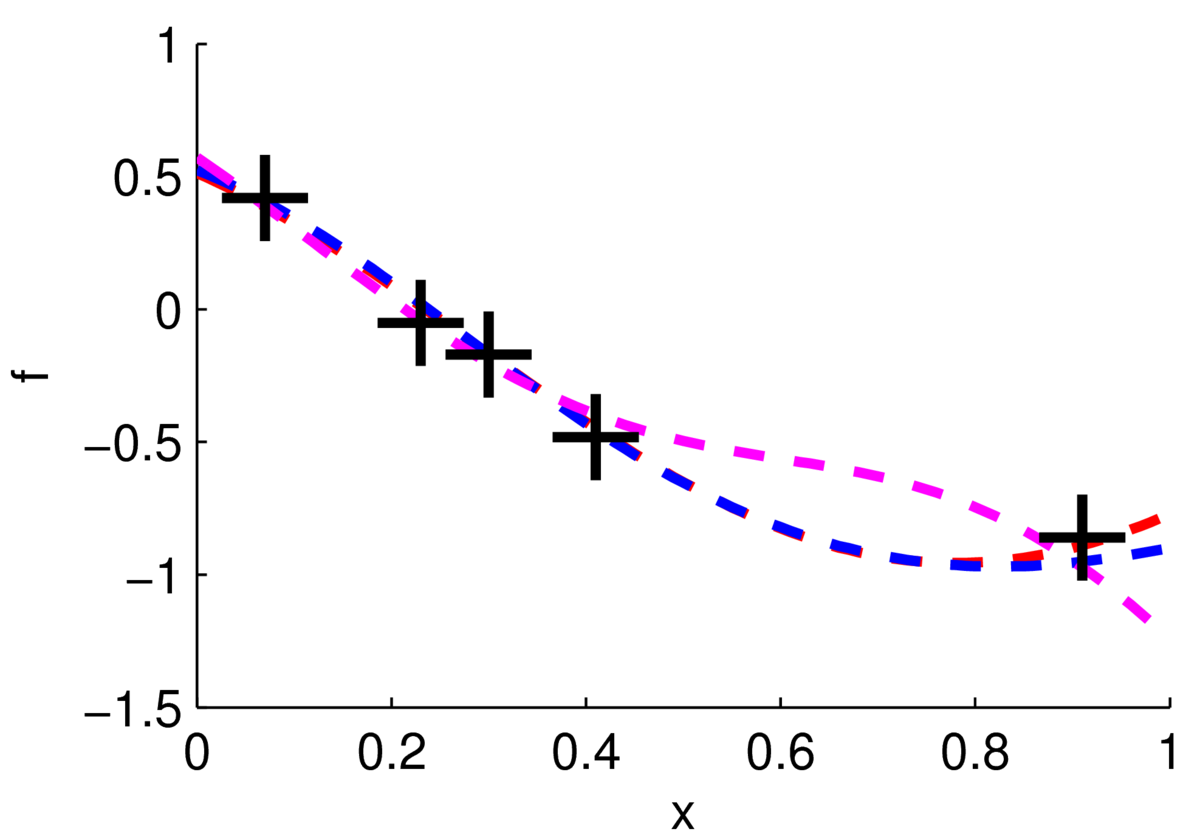
Really I plotted three samples from a 100-dimensional Gaussian, \(p(\bff_*\g \mathrm{data})\), where 100 test locations were chosen on a grid. We can see from these samples that we’re fairly sure about the function for \(x\in[0,0.4]\), but less sure of what it’s doing for \(x\in[0.5,0.8]\).
We can summarize the uncertainty at each input location by plotting the mean of the posterior distribution and error bars. The figure below shows the mean of the posterior plotted as a black line, with a grey band indicating \(\pm2\) standard deviations.
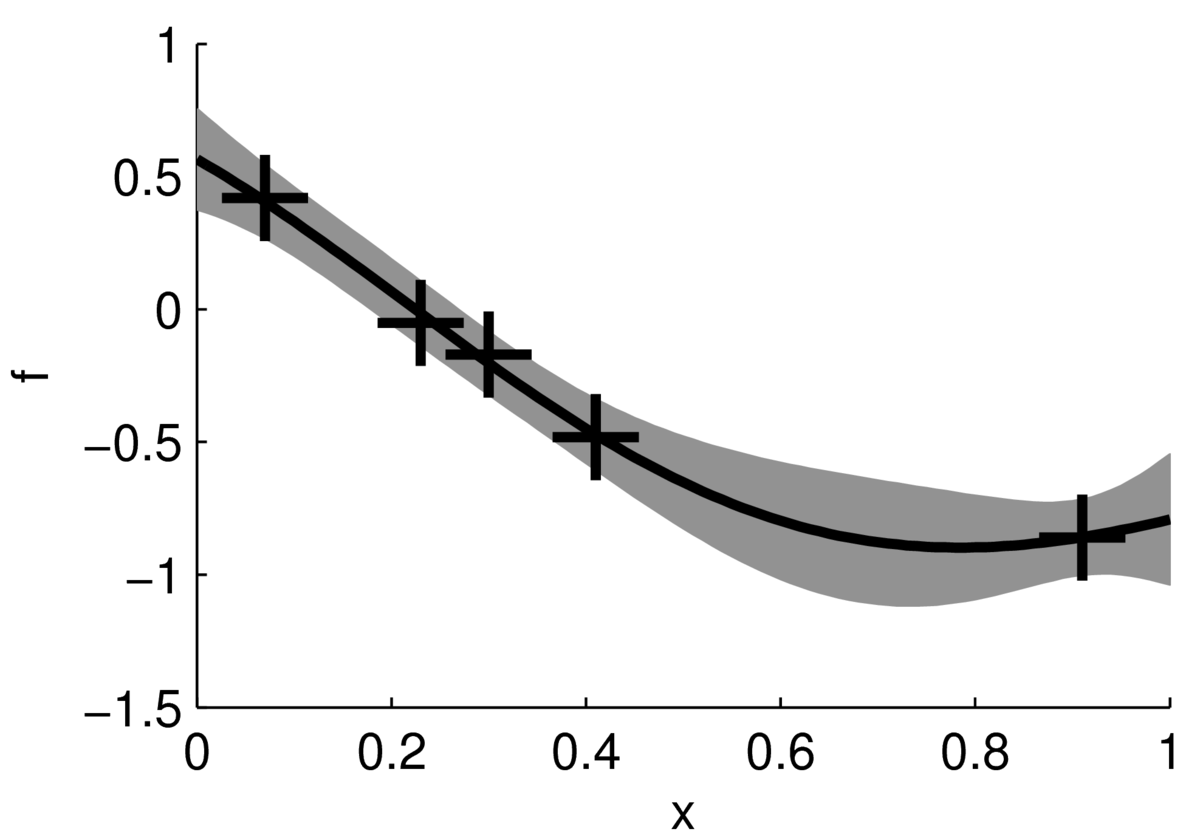
This figure doesn’t show how the functions might vary within that band, for example whether they are smooth or rough. However, it might be easier to read, and is cheaper to compute. We don’t need to compute the posterior covariances between test locations to plot the mean and error band. We just need the 1-dimensional posterior at each test point: \[
p(f(\bx^{(*)})\g \mathrm{data}) \,=\, \N(f;\; m,\, s^2).
\] To identify the mean \(m\) and variance \(s^2\), we need the covariances: \[
K_{ij} = k(\bx\ith, \bx\jth),\quad (\bk^{(*)})_i = k(\bx^{(*)}, \bx\ith).
\] Then the computation is a special case of the posterior expression already provided, but with only one test point: \[\begin{aligned}
M &= K + \sigma_y^2\eye,\\
m &= \bk^{(*)\top} M^{-1}\by,\\
s^2 &= k(\bx^{(*)}, \bx^{(*)}) - \underbrace{\bk^{(*)\top} M^{-1}\bk^{(*)}}_{\mbox{positive}}.
\end{aligned}
\] The mean prediction \(m\) is just a linear combination of observed function values \(\by\).
After observing data, our beliefs are always more confident than under the prior. The amount that the variance improves, \(\bk^{(*)\top} M^{-1}\bk^{(*)}\), doesn’t actually depend on the \(\by\) values we observe! These properties of inference with Gaussians are computationally convenient: we can pick experiments, knowing how certain we will be after getting its result. However, these properties are somewhat unrealistic. When we see really surprising results, we usually become less certain, because we realize our model is probably wrong. In the Gaussian process framework we can adjust our kernel function and noise model \(\sigma_y^2\) in response to the observations, and then our uncertainties will depend on the observations again.
What you should know
The marginal and conditional of a joint Gaussian are Gaussian. Be able to write down a marginal distribution given a joint.
GP idea: explain how a smooth curve or surface relates to a draw from a multivariate Gaussian distribution. How would you plot one?
Check your understanding
- Given a GP model and \(N\) observations in a regression task, what do you need to compute to predict the function value (with an error bar) at a test location? What is the computational cost of these operations? Would you actually be able to do it? Or is there anything else you need to know?
Reading
The core recommended reading for Gaussian processes is Murphy, Chapter 15, to section 15.2.4 inclusive.
Alternatives are: Barber Chapter 19 to section 19.3 inclusive, or the dedicated Rasmussen and Williams book up to section 2.5. There is also a chapter on GPs in MacKay’s book.
Gaussian processes are Bayesian kernel methods. Murphy Chapter 14 has more information about kernels in general if you want to read about the wider picture.
The idea of Bayesian optimization is old. However, a relatively recent paper rekindled interest in the idea as a way to tune machine learning methods: http://papers.nips.cc/paper/4522-practical-bayesian-optimization-of-machine-learning-algorithms These authors then formed a startup around the idea, which was acquired by Twitter. Other companies like Netflix have also used their software.
MLPR → Course Notes → w7c
PDF of this page
Previous: Bayesian model choice
Next: Gaussian Processes and Kernels
Notes by Iain Murray