The red dots are validation data: held out points that weren’t used to fit the curves. Training and validation errors were then plotted for polynomials of different orders:
You now have enough knowledge to be dangerous. You could read some data into matrices/arrays in a language like Matlab or Python, and attempt to fit a variety of linear regression models. They may not be sensible models, and so the results may not mean very much, but you can do it.
You could also use more sophisticated and polished methods baked into existing software. Many Kaggle competitions are won using the easy-to-use and fast XGBoost, or using ‘convolutional neural nets’, which you can fit with several packages, for example Keras.
How do you decide which method(s) to use, and work out what you can conclude from the results?
It is almost always a good idea to find the simplest possible algorithm that could possibly give an answer to your problem, and run it. In a regression task, you could report the mean square error of a constant function, \(f(x)\te b\). If you’re not beating that model on your training data, there is probably a bug in your code. If a fancy method does not generalize to new data as well as the baseline, then maybe the problem is simply too hard… or there are more subtle bugs in your code.
It is also usual to implement stronger baselines. For example, why use a neural network if straight-forward linear regression works better? If you are proposing a new method for an established task, you should try to compare to the existing state-of-the art if possible. (If a paper does not contain enough detail to be reproducible, and does not come with code, they may not deserve comparison.)
I’ve heard the following piece of advice for finding a machine learning algorithm to solve a practical problem1:
“Find a recent paper at a top machine learning conference, like NIPS or ICML that’s on the sort of task you need to solve. Look at the baseline that they compare their method to… and implement that.”
If they used a method for comparison, it should be somewhat sensible, but it’s probably a lot simpler and tested than the new method. And for many applications, you won’t actually need this year’s advance to achieve what you need.
We may wish to compare a linear regression model, \(f(\bx;\bw,b)=\bw^\top\bx + b\), to a constant function baseline \(f(\bx;b)=b\). The linear regression model can never be beaten on the training data by the baseline, even if the data are random noise. The models are nested: linear regression can become the simpler model by setting \(\bw\te\mathbf{0}\), and obtain the same performance. Then there will almost always be some way to set \(\bw\!\ne\!\mathbf{0}\) to improve the square error slightly.
Thus we cannot use the performance on a training set to pick amongst models. The most complicated model will usually win, and it will always win if the models are nested. Yet in the previous note we saw how dramatically bad the fit can be from models with many parameters.
Instead, we could compare our model to a baseline on a testing set or test set. The test data should have been held out when fitting or training the model. The test data is only used to report the square error the model achieves when generalizing to new data.
Formally, the generalization error, is the average error or loss that the model function \(f\) would achieve on future test cases coming from some distribution \(p(\bx,y)\): \[ \text{Generalization error} = \E_{p(\bx,y)}[L(y, f(\bx))] = \int L(y, f(\bx))\,p(\bx,y)\intd\bx\intd y, \] where \(L(y, f(\bx))\) is the error we record if we predict \(f(\bx)\) but the output was actually \(y\). For example, if we care about square error, then \(L(y, f(\bx)) = (y\tm f(\bx))^2\).
We don’t have access to the distribution of data examples \(p(\bx,y)\). If we did, we wouldn’t need to do learning! However, the average error on a test set of size \(M\), gives a Monte Carlo estimate of the integral above: \[ \text{Average test error} = \frac{1}{M} \sum_{m=1}^M L(y^{(m)}, f(\bx^{(m)})), \qquad \bx^{(m)},y^{(m)}\sim p(\bx,y). \] Assuming the test items are drawn from the distribution we are interested in, the expected value of the test error is equal to the generalization error. (Check you can see why.)
Reporting an average test error, rather than a total, usually means that the value is more interpretable, and the average error approaches a constant as the test set size \(M\) increases. For ease of comparison, I usually also report an average training error; I divide the sum of training errors across all cases by the number of training cases.
We shouldn’t evaluate many different alternative models on the test set. Selecting the best model from many variants often picks a model that did well by chance, so its test performance will often be lower on future data. For example, if we test a set of models with different regularization constants \(\lambda\) and select the best, we have fitted the parameter \(\lambda\) to the test set. However, the test set is meant for evaluation, and meant to be held-out from all training procedures.
Instead we should split the data that’s not held out for testing into a training set and validation set. We fit the main parameters of a model, such as the weights of a regression model on the training set. Different variants of the model, perhaps with different regularization parameters, are then evaluated on the validation set to see which settings seem to generalize best. Finally, to report how well the selected model is likely to do on future data, it is evaluated on the test set.
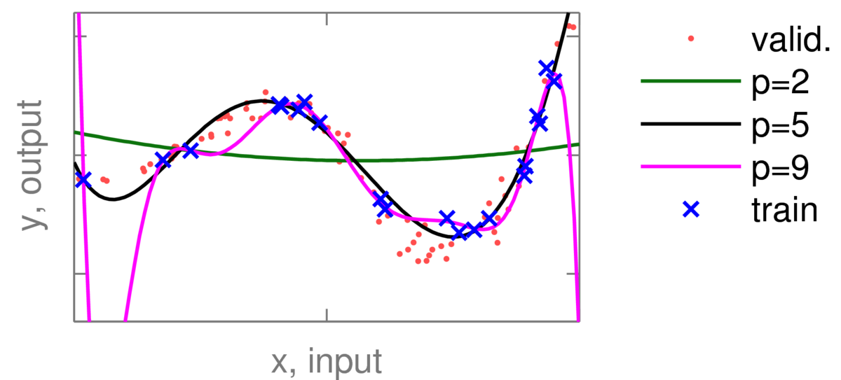
Example: the plot below shows some polynomial fits to some training data (blue crosses) with different degrees \(p\). The quadratic curve (\(p\te2\)) is under-fitting, and the 9th order polynomial is showing clear signs of over-fitting.
The red dots are validation data: held out points that weren’t used to fit the curves. Training and validation errors were then plotted for polynomials of different orders:
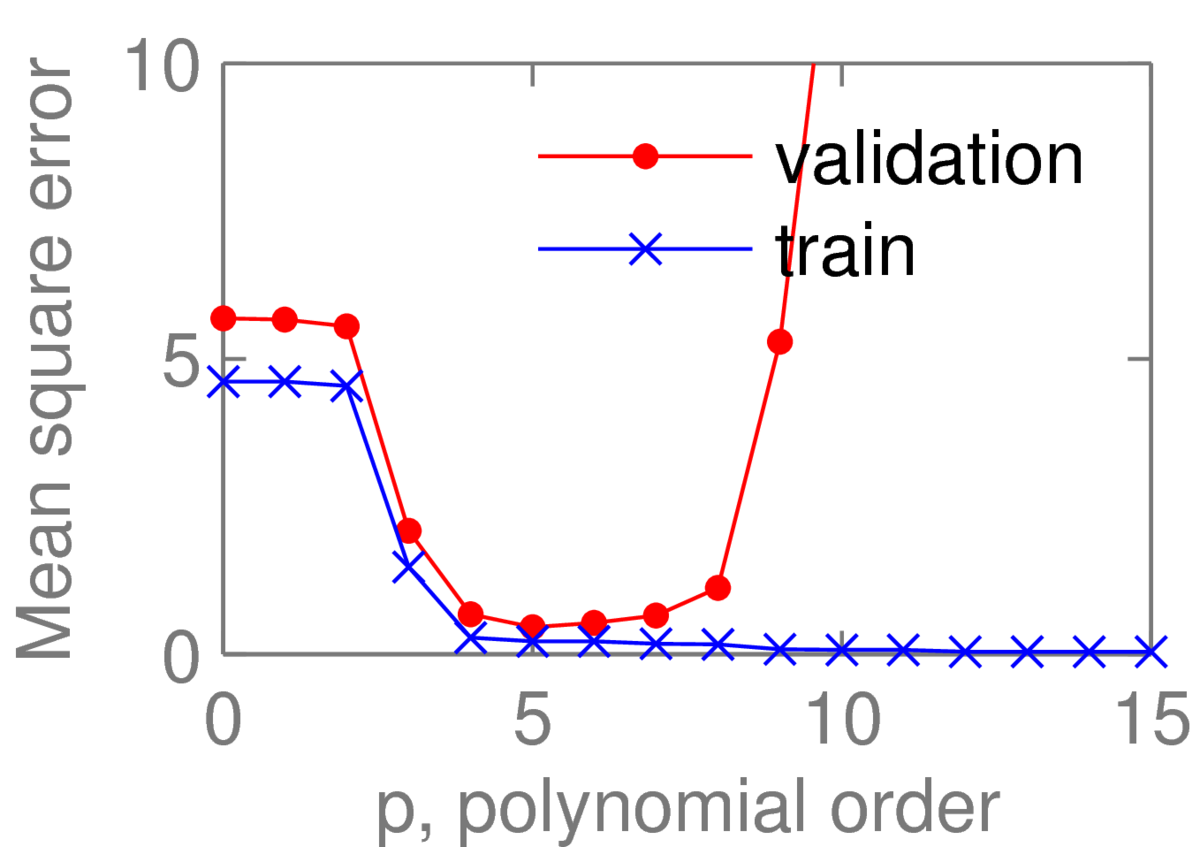
As expected for nested models, the training error falls monotonically as we increase the complexity of the model. However, the fifth order polynomial has the lowest validation error, so I might select that fit. Looking at the validation curve, the average error of the fourth to seventh order polynomials all seem similar. On reflection, I might instead pick the simpler fourth order polynomial.
How we should split up our data into the different sets? You might see papers that use (for example) 80% of data for training, 10% for validation, and 10% for testing. There’s no real justification for using any fixed set of percentages, but it’s likely that no one would question such a split. What we really want to do is use as much data for training as possible, so that we can fit a good model.2 We are limited by the need to leave enough data for validation and testing to choose models and report model performance. Deciding if we have enough validation/test data requires some statistics, which I’ll defer to a later note.
Given that we want to use as much data for training as possible, we could consider combining our training and validation sets after making model choices (basis functions, regularization constants, etc.) and refit. I don’t see this trick used often though, and usually avoid it in my research. Reason 1: If comparing to other work that uses a particular train/validation split, I try to stick to that. I don’t want to just get good numbers: I want a controlled comparison between models, so I can show that my numbers are better because of interesting differences between models. Reason 2: for models like neural nets, where an optimizer can find parameters in different regions on every run, I might be unlucky when refitting and fit a worse model. If I don’t have any validation data, I won’t notice.
A more elaborate procedure called \(K\)-fold cross-validation is appropriate for small datasets, where holding out validation data ‘just’ for the selection of model choices leaves too little data for training a good model. The data that we can fit to is split into \(K\) parts. Each model is fitted \(K\) times, each with a different part used as a validation set, and the remaining \(K\tm1\) parts used for training. We select the model with the lowest validation error, when averaged over the \(K\) folds.
Making statistically rigorous statements based on \(K\)-fold cross-validation performance is difficult. (Beyond this course and I believe an open research area.)
If there’s a really small dataset, a paper might report a \(K\)-fold score in place of a test set error. However, hyperparameters such as regularization constants should never be fitted to the measure used to report final performance. Therefore, any hyperparameters should either be set to default values, or set for each training fold using further cross-validation using only the training data in the current training fold. Performing so many model fits could be rather costly! Bayesian procedures (considered later in the course) can become especially appealing in these data-limited settings.
It is surprisingly easy to accidentally over-fit a model to the available test data, and then generalize poorly on future data. For example, someone may have followed good practice for all of their analysis, but then the final test score is disappointing. They then realize that there was something they should probably have done differently, so they change that and try again. Then they have another realization, but after that change the test score gets worse so they revert that change… and so on.
Each minor re-run of a method, or peek at the test set, doesn’t seem like it could cause any problems individually. But the effects build up. These problems with accidental over-fitting are frequently seen on Kaggle. Their competitions display a public leaderboard, based on a test set, but the final rankings are based on a second test set. It is common for some competitors to fall many places when the leaderboard is re-ranked. One such competitor wrote a reflective blog post on how they had fooled themselves. Despite knowing about cross-validation and the dangers of over-fitting, they slowly but surely slipped into fitting the test set. They reached second place on the public leaderboard, but fell dramatically when it was re-ranked… embarrassingly beneath one of the available baselines.
Training on the test set is one of the worst mistakes you can make in machine learning. At best, the results you present will be misleading, and at worst they will be meaningless. Markers of dissertation projects are likely to penalize such poor practice severely. In your own projects, if you can3, I suggest holding out some data that you never look at during the bulk of your research. Pretend it doesn’t exist. Then right at the end, test only the most-interesting models on the totally-held out test set.
Tests on held-out data provide straightforward quantitative comparisons between models. Based on these comparisons, if done properly, we can be fairly sure how well a model will generalize to data drawn from the same distribution.
Future data often won’t be drawn from the same distribution however. The properties of most systems drift over time. Dealing with these changes is hard, and often ignored. If your data is explicitly provided as a time-series, you may want to adopt a different training and testing procedure. For example, in online prediction, you predict each item one at a time in sequence, updating the model with each item after you have predicted it.
Even for stable systems, test set errors only say how well, under the given distribution, the models make predictions. A model with low test error does not necessarily reflect the structure of the real system, and as a result may generalize poorly if used in other ways. For example, you should be careful about attempting to interpret meaning behind the weights in a model. Statistics books are full of examples of how various problems (e.g., selection effects, confounds, and model mismatch) can make you reach completely wrong conclusions about a system from a model’s fitted parameters.
Can you show that the test error is an unbiased estimate of the generalization error? That is, that the expected value of the test error is equal to the generalization error.
Recall and explain why the training error can’t go up as we increase the order of the polynomials we are fitting. A good explanation would be understandable by another student who has not yet read this note.
You should now be able to write some simple code to pick an L2 regularizing constant when (for example) fitting a regression problem with a fixed set of RBF basis functions. You could produce figures like the ones in this note. In a paper, or on an exam, you might have to explain such a procedure in English, or pseudo-code.
Could you adapt your procedure to fit both a regularizing constant, and a width \(h\) shared by a set of RBF basis functions? What difficulties do you face as the number of hyper-parameters that you want to set grows? Would you have difficulty setting separate centres and/or widths for each RBF?
How many model settings would we have to fit if we do \(K\)-fold cross-validation to select a regularization constant for a model?
If our final report of a model’s performance is going to be a \(K\)-fold cross-validation score, we might do a further \(K\)-fold cross-validation on each training fold to set hyper-parameters. Can you explain why? How many models will we end up fitting?
The following two book sections contain more (optional) details. These sections may assume some knowledge we haven’t covered yet.
Keen students could read the following book chapter by Amos Storkey: When training and test sets are different: characterising learning transfer. In Dataset Shift in Machine Learning, Eds Candela, Sugiyama, Schwaighofer, Lawrence. MIT Press.
These notes described over-fitting as producing unreasonable fits that will generalize poorly, at the expense of fitting the training data unreasonably closely. Thus, models that are said to over-fit usually have lower training error than ‘good’ fits, yet higher generalization error.
I believe it is hard to crisply define over-fitting however. Mitchell’s Machine Learning textbook (1997, p67) attempts a definition:
“A hypothesis \(f\) is said to over-fit the data if there exists some alternative hypothesis \(f'\) such that \(f\) has a smaller training error than \(f'\), but \(f'\) has a smaller generalization error than \(f\).”
However, I think almost all models \(f\) that are ever fitted would satisfy these criteria! Thus the definition doesn’t seem useful to me.
If we thought we have enough data to get a good fit to a system everywhere, then we would expect the training and validation errors to be similar. Thus a possible indication of over-fitting is that the average validation error is much worse than the average training error. However, there is no hard rule here either. For example, if we know that our data are noiseless, we know exactly what the function should be at our training locations. It is therefore reasonable we will get lower error at or close to the training locations than at test locations in other places.
I have seen people reject a model with the best validation error because it’s “over-fitting”, by which they mean the model had a bigger gap between its training and validation score than other models. Such a decision is misguided. It’s the validation error that gives an indication of generalization performance, not the difference between training and validation error. Moreover, it’s common not to have enough data to get a perfect fit everywhere. So while it’s informative to inspect the training and validation errors, we shouldn’t insist they are similar.
The reality is that there is no single continuum from under-fit models to over-fit models, that passes through an ideal model somewhere in between. I believe most large models will have some aspects that are overly simplified, yet other aspects that result from an unreasonable attempt to explain noise in the training items.
While I can’t define over-fitting precisely, the concept is still useful. Adding flexibility to models does often make test performance drop. It is a useful shorthand to say that we will select a smaller model, or apply a form of regularization, to prevent over-fitting.
I wish I knew who to credit. The “quote” given is a paraphrase of something I’ve heard in passing.↩
In the toy example above, I artificially used a small fraction of the data for training so that we’d quickly get over-fitting for demonstration purposes.↩
Sometimes this best practice is hard to realize.↩