The costs of some classifiers:
We have a training set of \(N\) examples, with \(D\)-dimensional features and binary labels. This question gets you to revisit what computations you need to do to build and use a classifier.
Assume the following computational complexities: matrix-matrix multiplication \(AB\) costs \(O(LMN)\) for \(L\ttimes M\) and \(M\ttimes N\) matrices \(A\) and \(B\). Inverting an \(N\ttimes N\) matrix \(G\) and/or finding its determinant costs \(O(N^3)\).2
What is the computational complexity of training a “Bayes classifier” that models the features of each class by a maximum likelihood Gaussian fit (a Gaussian matching the mean and covariances of the features)?
What is the computational complexity of assigning class probabilities to a test feature vector?
In linear discriminant analysis we assume the classes just have different means, and share the same covariance matrix. Show that given its parameters \(\theta\), the log likelihood ratio for a binary classifier, \[\notag \log \frac{p(\bx\g y\te1,\,\theta)}{p(\bx\g y\te0,\,\theta)} \;=\; \log p(\bx\g y\te1,\,\theta) - \log p(\bx\g y\te0,\,\theta), \] is a linear function of \(\bx\) (as opposed to quadratic).
When the log likelihood ratio is linear in \(\bx\), the log posterior ratio is also linear. Reviewing Q3 in tutorial 4, we can recognize that when the log posterior ratio is linear, the predictions have the same form as logistic regression: \[\notag P(y\te1\g\bx,\,\theta) = \sigma(\bw^\top\bx + b), \] but the parameters \(\bw(\theta)\) and \(b(\theta)\) are fitted differently.
How do your answers to a) and b) change when the classes share one covariance? What can you say about the cost of the linear discriminant analysis method compared to logistic regression?
Gradient descent:
Let \(E(\bw)\) be a differentiable function. Consider the gradient descent procedure \[\notag \bw^{(t+1)} \leftarrow \bw^{(t)} - \eta\nabla_\bw E. \]
Are the following true or false? Prepare a clear explanation, stating any necessary assumptions:
Let \(\bw^{(1)}\) be the result of taking one gradient step. Then the error never gets worse, i.e., \(E(\bw^{(1)}) \le E(\bw^{(0)})\).
There exists some choice of the step size \(\eta\) such that \(E(\bw^{(1)}) < E(\bw^{(0)})\).
A common programming mistake is to forget the minus sign in either the descent procedure or in the gradient evaluation. As a result one unintentionally writes a procedure that does \(\bw^{(t+1)} \leftarrow \bw^{(t)} + \eta\nabla_\bw E.\) What happens?
Maximum likelihood and logistic regression:
Maximum likelihood logistic regression maximizes the log probability of the labels, \[\notag \sum_n \log P(y^{(n)}\g \bx^{(n)}, \bw), \] with respect to the weights \(\bw\). As usual, \(y^{(n)}\) is a binary label at input location \(\bx^{(n)}\).
The training data is said to be linearly separable if the two classes can be completely separated by a hyperplane. That means we can find a decision boundary \[\notag P(y^{(n)}\te1\g \bx^{(n)}, \bw,b) = \sigma(\bw^\top\bx^{(n)} + b) = 0.5,\qquad \text{where}~\sigma(a) = \frac{1}{1+e^{-a}},\] such that all the \(y\te1\) labels are on one side (with probability greater than 0.5), and all of the \(y\!\ne\!1\) labels are on the other side.
Show that if the training data is linearly separable with a decision hyperplane specified by \(\bw\) and \(b\), the data is also separable with the boundary given by \(\tilde{\bw}\) and \(\tilde{b}\), where \(\tilde{\bw} \te c\bw\) and \(\tilde{b} \te cb\) for any scalar \(c \!>\! 0\).
What consequence does the above result have for maximum likelihood training of logistic regression for linearly separable data?
Logistic regression and maximum likelihood: (Murphy, Exercise 8.7, by Jaaakkola.)
Consider the following data set:
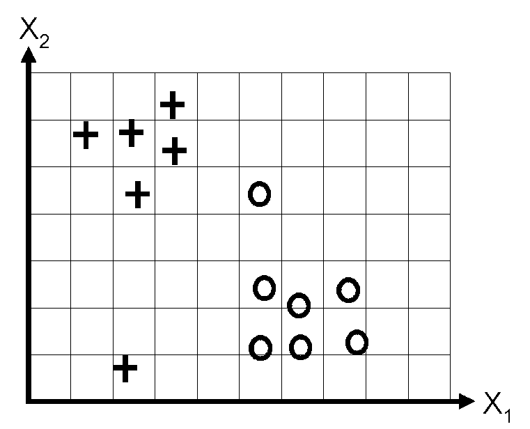
Suppose that we fit a logistic regression model with a bias weight \(w_0\), that is \(p(y \te 1\g \bx, \bw) = \sigma(w_0 + w_1 x_1 + w_2 x_2 )\), by maximum likelihood, obtaining parameters \(\hat{\bw}\). Sketch a possible decision boundary corresponding to \(\hat{\bw}\). Is your answer unique? How many classification errors does your method make on the training set?
Now suppose that we regularize only the \(w_0\) parameter, that is, we minimize \[\notag J_0(\bw) = -\ell(\bw) + \lambda w_0^2, \] where \(\ell\) is the log-likelihood of \(\bw\) (the log-probability of the labels given those parameters).
Suppose \(\lambda\) is a very large number, so we regularize \(w_0\) all the way to 0, but all other parameters are unregularized. Sketch a possible decision boundary. How many classification errors does your method make on the training set? Hint: consider the behaviour of simple linear regression, \(w_0 + w_1 x_1 + w_2 x_2\) when \(x_1 \te x_2 \te 0\).
Now suppose that we regularize only the \(w_1\) parameter, i.e., we minimize \[\notag J_1(\bw) = -\ell(\bw) + \lambda w_1^2. \] Again suppose \(\lambda\) is a very large number. Sketch a possible decision boundary. How many classification errors does your method make on the training set?
Now suppose that we regularize only the w2 parameter, i.e., we minimize \[\notag J_2(\bw) = -\ell(\bw) + \lambda w_2^2. \] Again suppose \(\lambda\) is a very large number. Sketch a possible decision boundary. How many classification errors does your method make on the training set?