MLPR → Course Notes → w3a
PDF of this page
Previous: Multivariate Gaussians
Next: Regression and Gradients
$$
\newcommand{\E}{\mathbb{E}}
\newcommand{\N}{\mathcal{N}}
\newcommand{\bm}{\mathbf{m}}
\newcommand{\bmu}{{\boldsymbol{\mu}}}
\newcommand{\bx}{\mathbf{x}}
\newcommand{\by}{\mathbf{y}}
\newcommand{\g}{\,|\,}
\newcommand{\te}{\!=\!}
\newcommand{\tm}{\!-\!}
$$
Classification: Regression, Gaussians, and pre-processing
So far we have fitted scalar real-valued functions \(f(\bx)\) from a real-valued input vector \(\bx\). We have matched these to real-valued observations or targets \(y\), a task often called regression. However, the inputs and outputs of the function we wish to learn could take different types. This note begins to look at some of the alternatives.
The most common machine learning task is probably classification. We have a dataset of inputs and outputs, \(\{\bx^{(n)}, y^{(n)}\}\) as before, but the \(y\) labels now belong to a discrete set of categories. In binary classification, \(y\) takes on one of only two values, often \(\{0,1\}\) or \(\{-1,+1\}\), for example indicating if an email is spam or not, or an image contains a particular object of interest or not.
There are many different ways we could represent and learn a function that predicts discrete labels. This note gives some of the different ways to represent the function. We will extend these, and say a lot more about learning later in the course.
Just do regression?
Although the labels in classification problems are discrete, \(0\) and \(1\) are still numbers. We could take a training set for a binary classification problem, and use it to fit a linear regression model where all of the outputs just happen to be \(0.0\) and \(1.0\). Is that a good idea?
Given enough basis functions, and data to fit them, we can get a fit close to any function, so we could fit a function that takes on values close to \(0\) and \(1\) for most of its inputs. What if the labels are noisy, and we can observe both zeros and ones in the same location? Then to minimize square error, the best function value at a location where \(p(y\te1)\te p_1\) would minimize: \[
\E[(y-f)^2] = p_1(1\tm f)^2 + (1\tm p_1)(0\tm f)^2 = f^2 -2p_1f + p_1,
\] which is minimized by \(f\te p_1\). So in the limit of lots of basis functions and data, a flexible linear regression model can give the probability that a binary label \(y\!\in\!\{0,1\}\) will be one. If we wanted to pick the most probable class, we would return one if our function was greater than a half, and zero otherwise.
As we can fit regularized least squares regression models quickly, and with very little code, regressing the labels can be appealing. On the other hand, for a fixed set of basis functions, it is easy to find examples where the least squares objective does not return the most useful function for constructing a classification rule. See if you can sketch one, before I show you an example.
Also, regardless of how we fit a linear regression model, the fitted functions will usually extend outside \(f\!\in\![0,1]\) for some inputs, which makes it hard to take the probabilistic interpretation seriously.
What follows is code to construct an example showing a limitation of least squares fitting. It shows (in magenta) a least squares quadratic fit to some data, and (in black) another quadratic curve, which when thresholded at 0.5, is a much better classifier.
Matlab:
% Train model on synthetic dataset
N = 200;
X = rand(N, 1)*10;
yy = double((X > 1) & (X < 3));
phi_fn = @(X) [ones(size(X,1),1) X X.^2];
ww = phi_fn(X) \ yy;

% Predictions
x_grid = (0:0.05:10)';
f_grid = phi_fn(x_grid)*ww;

% Predictions with alternative weights:
w2 = [-1; 2; -0.5]; % Values set by hand
f2_grid = phi_fn(x_grid)*w2;

% Show demo
clf; hold on;
plot(X(yy==1), yy(yy==1), 'r+')
plot(X(yy==0), yy(yy==0), 'bo')
plot(x_grid, f_grid, 'm-')
plot(x_grid, f2_grid, 'k-')
ylim([-0.1, 1.1])
Python:
import numpy as np
import matplotlib.pyplot as plt

# Train model on synthetic dataset
N = 200
X = np.random.rand(N, 1)*10
yy = (X > 1) & (X < 3)
def phi_fn(X):
    return np.concatenate([np.ones((X.shape[0],1)), X, X**2], axis=1)
ww = np.linalg.lstsq(phi_fn(X), yy)[0]

# Predictions
x_grid = np.arange(0, 10, 0.05)[:,None]
f_grid = np.dot(phi_fn(x_grid), ww)

# Predictions with alternative weights:
w2 = [-1, 2, -0.5] # Values set by hand
f2_grid = np.dot(phi_fn(x_grid), w2)

# Show demo
plt.clf()
plt.plot(X[yy==1], yy[yy==1], 'r+')
plt.plot(X[yy==0], yy[yy==0], 'bo')
plt.plot(x_grid, f_grid, 'm-')
plt.plot(x_grid, f2_grid, 'k-')
plt.ylim([-0.1, 1.1])
plt.show()
Remember: I’m not saying we can’t use linear regression for classification. We could fit the problem above by using more basis functions. However, for a fixed model and data-set, linear regression may generalize worse than other approaches. Linear regression could still be a baseline for comparison (although by the end of the course, you might jump straight to other baselines).
[We will soon, but not in this note, cover logistic regression, which is one way of forcing the function that we are fitting to lie between zero and one.]
‘One-hot’ or ‘one-of-\(K\)’ encodings
What about problems with more than two classes? We might classify a book into one of a set of categories: \(\{\texttt{crime}, \texttt{sport}, \texttt{fantasy}, \ldots\}\). We could index these classes with integers (e.g., \(y\te2\) implies \(\texttt{sport}\)). However, for a linear model, we would be insisting that a book whose feature vector is the average of the vector for a crime novel and the vector for a fantasy novel will be about sport(!).
An alternative numerical representation of a categorical variable uses a binary vector. Every element is zero, except for a single one, indicating which class is present. For example, we can indicate the 2nd class (e.g., \(\texttt{sport}\)) with the vector \(\by = [0~1~0~0~\ldots]^\top\). We could then fit a separate regression model to each element of the vector, and predict the label of a test input by reporting the class whose regression function gives the largest value.
Because expanding a discrete label into a binary vector is a common trick, there is jargon for it. It’s commonly called ‘one-hot’, ‘one-of-\(K\)’, or ’one-of-\(M\)’ encoding. I’m sure it has other names as well.
One-hot encoding the discrete input features in \(\bx\) can also be a good idea. If fitting a linear model to predict the popularity of a book, there’s probably no reason to assume that the predictions for sport should be between those of crime and fantasy.
Simple generative models
Another way to build a classifier is to fit a simple model of each class. Like linear regression, the fitting code can be short and quick, so these classifiers are good as baselines.
For real-valued input features, we could assume (almost certainly incorrectly) that the feature-vectors for each class come from a Gaussian distribution: \[
p(\bx\g y\te k) = \N(\bx; \bmu_k, \Sigma_k).
\] The simplest procedure is to fit the mean and covariance of Gaussian \(k\) to the mean and covariance of the feature vectors we have seen where the corresponding label was \(k\).
We can then use Bayes’ rule to invert this model, and ask what the model believes about the label, given a setting of the features: \[\begin{aligned}
P(y\te k\g \bx) &\propto p(\bx\g y\te k)\,P(y\te k) \\
&\propto \N(\bx; \bmu_k, \Sigma_k)\,\pi_k.
\end{aligned}\] For this instance of Bayes’ rule, the ‘prior distribution’ \(P(y)\) indicates how frequently we think the different labels will be used.
We might simply estimate the probabilities of the labels using counts: \[
P(y\te k) = \pi_k \approx \frac{\sum_n I(y^{(n)} = k)}{N},
\] where \(I\) is an indicator returning one or zero.
At training time we fit the model parameters, \(\theta \te \{\bmu_k,\Sigma_k,\pi_k\}\). That is easy: measure some means, covariances, and fractions, which are all based on simple averages over the dataset. Then at test time, given an input \(\bx\), we can compute a score for each class, \[
s_k = \N(\bx; \bmu_k, \Sigma_k)\,\pi_k
\] and normalize it to give a distribution over the labels: \[
P(y\te k\g \bx, \theta) = \frac{s_k}{\sum_{k'} s_{k'}}.
\] Here I’ve been explicit in saying that the probability is conditioned on a set of parameters \(\theta\). When first introducing the model above I left it implicit that the probabilities depended on some model settings. In papers and books you’ll often find probabilities that are implicitly conditioning on things that have been dropped from the notation.
The scatter plot below shows two features for 569 preparations of cells from the Wisconsin Breast Cancer Data at the UCI machine learning repository.
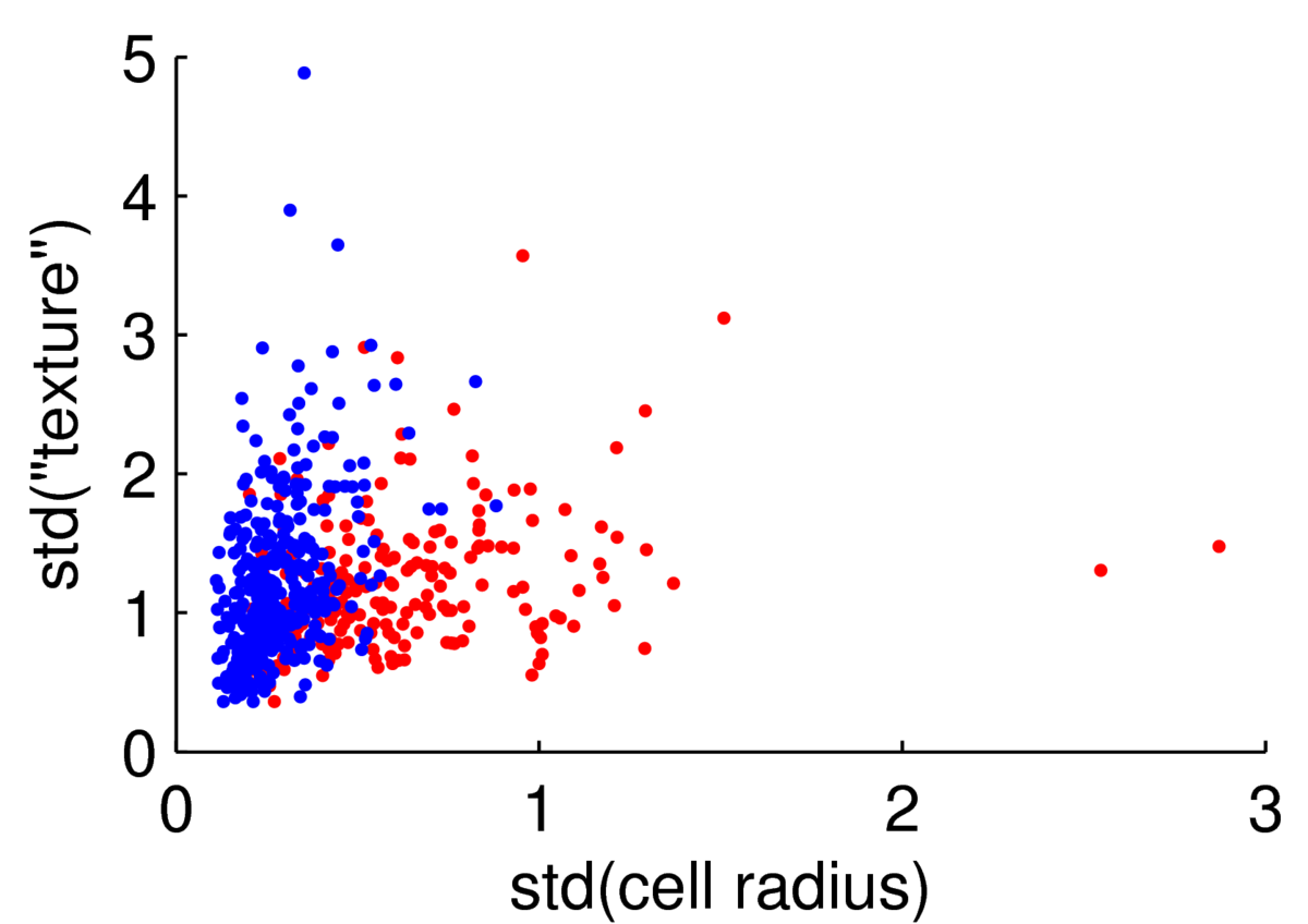
We could attempt to fit a multivariate Gaussian to the blue points (normal cells), another to the red points (malignant cells), to fit a simple classifier. However, the points are clearly not from a Gaussian distribution. The features are always positive, and Gaussian models would put probability mass on negative values. Whenever I have positive data, I consider taking its logarithm. As often happens, taking logs gives a scatter plot that is easier to read, and has more-plausibly Gaussian-shaped clouds:
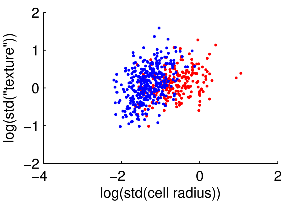
Hopefully if we looked at more features these clouds could be separated rather more than they are here.
Warning: you would need to think hard about the application and how the data were sampled before possibly trusting a classifier in an application that matters. Medical applications are particularly sensitive. One flaw with fitting a classifier as outlined above is that half of patients do not have cancer. This classifier would give quite high probabilities of cancer to every test example, which would be impractical to act on and could cause needless worry. More subtle problems could depend on exactly how the patients in the training set were selected within each class, and whether those choices will be reflected at test time.
“Bayes classifiers” and “Naive Bayes”
The Gaussian classifier above is an example of what is often called a “Bayes Classifier”. A model is built for each class and then Bayes’ rule is used at test time to form a distribution over classes.
For discrete features, we could fit a discrete probability distribution for each class, instead of the Gaussians. There isn’t a correlated, multivariate distribution of discrete features that’s as easy to deal with as the Gaussian. Instead it’s common to fit a model that assumes the features are independent. For binary features, \(x_d\!\in\!\{0,1\}\) the assumption can be written as: \[ P(\bx\g y\te
k, \theta) = \prod_d P(x_d\g y\te k,\theta) = \prod_d
{\theta_{d,k}}^{x_d}(1-\theta_{d,k})^{1-x_d}, \] where \(\theta_{d,k}\) gives the probability that \(x_d\te1\) given that the class is \(k\). The assumption that the features are independent given the class is known as the Naive Bayes assumption. Not all Bayes Classifiers are “Naive”! How would we restrict the Gaussian classifier above to make it a Naive Bayes Classifier?
Warning about a common confusion: Later in the course we will cover “Bayesian methods”. These use Bayes’ rule to express beliefs about the parameters of a model given some training data. For example, we don’t really know the distribution of the features of malignant cells exactly, we just have an estimate from a finite data set. Bayesian methods keep track of the uncertainty we have in our model throughout the analysis. Confusingly, the “Bayes classifiers” described in this document—which simply fit parameters and then assume them to be correct—are not “Bayesian methods” in the sense that is normally meant!
This document covered a couple of approaches to classification: least squares linear regression, and Bayes classifiers. However, just as important in practice, if not more so, are the pre-processing methods: one-hot/one-of-\(K\) encoding and log-transformations.
Bayes classifiers are a basic work-horse of practical machine learning. However, I didn’t want to spend a lot of time on examples in this course. Naive Bayes in particular already occurs in several undergraduate Edinburgh courses, and probably undergraduate courses in many other Universities. However, if you haven’t seen Naive Bayes before, I suggest you read more about it. It’s a good baseline to try, and easy to run on enormous datasets. However, you should know that the probabilities reported by Naive Bayes classifiers are usually poorly calibrated, caused by its strong and wrong independence assumptions. It’s possible to construct synthetic examples where Naive Bayes is either overly-confident, or under-confident. Keen students could try to do so. In text classification, Naive Bayes is usually extremely overconfident.
Check your understanding
Sketch a dataset with binary labels where a Gaussian Bayes classifier would work well, but a Gaussian Naive Bayes classifier would not.
Sketch a dataset with binary labels where a Gaussian classifier would not work well, but some other classifier could work.
Further Reading
I don’t think Murphy or Barber cover the idea of using least squares linear regression for binary classification. They go straight to the more sophisticated logistic regression method when modelling binary outputs. You can find discussion in Bishop (Section 4.1.3, p184), or the classic Duda and Hart Pattern Classification book (Section 5.8 in the Duda, Hart and Stork second edition from 2000). A book that’s free online, which dives straight into the multiple class case with one-hot encoding, is Hastie et al.’s The Elements of Statistical Learning (Section 4.2 in both the 1st and 2nd editions). The Rasmussen and Williams book Gaussian Processes for Machine Learning is also free online, and covers this idea in Section 6.5 (we will discuss Gaussian Processes later in the course).
Murphy has more detail on Bayes classifiers in section 3.5, and Gaussian classifiers in section 4.2. Barber covers Naive Bayes in Chapter 10, and a classifier based on a mixture of Gaussians (a generalization we haven’t covered yet) in 20.3.3.
MLPR → Course Notes → w3a
PDF of this page
Previous: Multivariate Gaussians
Next: Regression and Gradients
Notes by Iain Murray