Lab 2: Exploring corpus data with Python and matplotlib
| Author: | Sharon Goldwater |
|---|---|
| Date: | 2014-09-01, updated 2015-10-01, 2017-09-15, 2018-08-20, 2019-09-18 |
| Copyright: | This work is licensed under a Creative Commons Attribution-NonCommercial 4.0 International License: You may re-use, redistribute, or modify this work for non-commercial purposes provided you retain attribution to any previous author(s). |
This lab is available as a web page or pdf document.
Goals and motivation of this lab
In Lab 1 we saw that you can do some basic exploration of language data using only UNIX commands, but in general you will want to go further. Using Python we can write more complex functions that process multiple files, and we will also see how to visualize the data using Matplotlib library functions. We have also included several questions to get you thinking about the linguistic data and what it means, which is important even if you already know how to do the programming parts!
The example functions and plots used in this lab will start to give you a basis for lots of other functions and plots you may need to write later, either for homework assignments in this class, for other classes, or for your projects over the summer. (These really are only a start; we'll continue developing more plotting skills next week.)
Because some students are still Python beginners, we have written most of the code here already and have added a lot of comments explaining how it works. You'll have a chance to modify some of the code to help you understand it better.
For students who are more experienced programmers: please note that we have tried to keep the coding style here very simple, and have avoided some of the more advanced language features of Python. However, see the 'Going Further' section at the end if you want to try your hand at using some of those features.
Preliminaries
This lab will be using the same data set as Lab 1. If you didn't download the data already, please do so following the instructions in Creating your lab directory and Downloading the data from Lab 1. Below we will assume the data is located in your lab1 directory.
Now, create a directory for this lab inside the labs directory you made last week (or in the previous step) and cd into that directory:
cd ~/anlp/labs
mkdir lab2
cd lab2
Download the file lab2.py into your lab2 directory: From the Lab 2 web page, right-click on the link and select Save link as..., then navigate to your lab2 directory to save.
Running the code using Spyder and iPython
As you may already know, there are different ways to edit and run Python code. In this class, we will use the Spyder IDE, based on the iPython interpreter. To start the IDE, just type the following into a terminal:
spyder3 &
You'll get a new full-screen window, with a text editor on the left and two smaller sub-windows on the right: A Usage note on top and an iPython console below, running Python version 3.6.
Using the tabs at the bottom edge of the top one, change it to the Variable explorer view.
In the iPython console you should see a In [1]: prompt, and can now do things like this (where the Out line is the interpreter's response):
In [1]: 3+4
Out[1]: 7
Now open lab2.py in the editor (File -> Open...) and take a quick look at it. You will see that there are some import statements at the top; if you are new to Python you should read the comments in the code that explain what they do, though you need not do so right now. (Comments are enclosed in triple quotes ''' or begin with a hash mark #.)
In the main part of the file there are several function definitions, which we will explore in more detail in the rest of the lab, and a block of code that gets command line arguments and calls the functions, as we'll explain in a moment.
Now, run the code by typing the following into the interpreter:
cd ~/anlp/labs/lab2
%run lab2.py
(Note: commands that start with '%' are specific to iPython, and may not work in other Python interpreters. Similarly, iPython allows you to use Unix commands such as ``cd`` and tab completion, which may not work in other interpreters.)
What happened? Can you see which line of code in lab2.py generated the message you got?
You can also run the code from the terminal. Verify this by typing the following in a terminal window:
python lab2.py
You should see the same message you got before. But, the advantage of using %run with iPython is that after running the code, we still have access to all the variables and functions defined in it, which we do not have if we run the code in the terminal. To see how this works, go back to the interpreter and try this:
%run lab2.py ../lab1/Providence/Ethan/eth01.cha ../lab1/Providence/Ethan/eth02.cha
Remember you can use tab completion to avoid typing as much.
You should see a plot pop up on the screen. We will come back to the plot in a moment, so for now just close that window (otherwise you will not be able to type anything further into the interpreter).
Since you now have access to the variables defined in lab2.py, try typing fnames in the interpreter. What is the value of this variable?
In case you are wondering, fnames was set using the special variable sys.argv, which gets set automatically to be the list of arguments provided at the terminal or %run command (with sys.argv[0] being the program name, here lab2.py, and the rest of the items in the list being any remaining arguments, in this case the filenames).
Now, without looking at the value of the word_counts variable, can you figure out what data type it is? (Hint: look at the comments and/or code in the ``get_word_counts`` function.).
Once you have figured that out, you should be able to get the count of the word 'the'. What is it?
Notice that you can also find word_counts in the Variable explorer window, where you can double click on the word_counts variable to see the whole dictionary.
So far we ran code in the interpreter using %run. But you can also run code using the Spyder menus. To do this, set Command line options in Run -> Configure.. to ../lab1/Providence/Ethan/eth01.cha ../lab1/Providence/Ethan/eth02.cha and then click the green arrow button on the main menu bar.
In the remainder of the lab we run code using %run, but you can run them with the Spyder menu if you prefer.
Getting help in iPython (and in general)
Before moving on, let's make sure you know how to get help. There are several ways to do this:
Simply type help() at the iPython interpreter prompt; you can then type a module name (e.g., string) and you will get some documentation. Actually a lot of documentation, but maybe not the most helpful kind. So, it may be better to try options 2 or 3. (Hit q to exit help.)
To get a list of all the methods available for a particular variable, you can use tab completion in iPython. This can also work to tell you all the methods available for particular datatype, like a string. For example, type the following two lines into the interpreter, but don't hit <enter> after the second line:
ss = "a string"
ss.
Now type <tab>. You should see a list of all of the methods you can call on ss, which is to say, all the methods for strings.
- Often it's most appropriate to just search the Internet, if you want more general information, don't know the name of the function you're looking for, want examples of how to use particular functions, or whatever.
- A final point: help also works for functions defined in your own code, if you have written documentation for them. Try typing help(zipf_plot). Notice where the documentation comes from in the code we wrote in lab2.py.
Looking at the data
The code we have given you is actually not quite correct. Let's try to figure out what is wrong and how to fix it. First, create a plot like the one we saw before but this time using only one file:
%run lab2.py ../lab1/Providence/Ethan/eth01.cha
First, compare the left-hand (linear) and right-hand (log) plots. Notice that on the linear plot it is nearly impossible to see what's going on except for the very top-ranked words. Those words are so much more frequent than anything else that on the linear axes, almost all the words are compressed into a tiny portion of the plot. You will also see that there are huge differences in frequency between the top few words; as you look further down the list, closely ranked words have more similar frequencies.
Do you see anything funny in the Zipf plot? If you're not sure yet, try checking some of the following. These are all good things to sanity check whenever you are looking at language data:
How many unique word types are there? (Use the len function).
What are the first few and last few words as sorted alphabetically? (Use the sorted function and list indexing to look at only part of the list)
What are the first few and last few words as sorted by frequency? (To sort the keys in a dictionary, say mydict, according to the values of the keys, you can do this:
sorted(mydict, key=mydict.get)
Create your own tiny dictionary called mydict to verify this.)
- If you have some previous programming/Python experience (don't try this otherwise), an even better thing to do is to modify the zipf_plot function so that the words themselves show up as the x-axis labels. You'll need to use the xticks function from matplotlib (Google it), and you can zoom in on just the top-ranked words by using the optional maxRank argument to zipf_plot. (Of course, this won't help you debug anything that's wrong with lower ranked words).
Hopefully by this time you will have noticed some problems with the data in word_counts. If you re-create the Zipf plot, can you see where these problems are showing up?
Fixing the problem
Now that you have identified what's wrong with word_counts, you should be able to make some very small changes to the get_word_counts function that fix the problems, at least mostly. There may still be a few things in word_counts that you don't consider real words. What are some of those things? [The question of what counts as a word and what doesn't comes up a lot in NLP, and there is rarely a single correct answer; often we need to use our judgment and justify our decisions.]
After making your changes to get_word_counts, re-run the code. Does the plot look any better now? Go back and do the sanity checks in the previous section again to make sure you didn't miss anything else. You can also try running the code with a larger number of files, e.g.:
%run lab2.py ../lab1/Providence/Ethan/eth*.cha
The plot should look similar but smoother than it does with only one or two files. Why is it smoother?
MLU
Before going further, take a look at the get_mlus function and make sure you understand what it is doing. What do the variables ntoks and nutts represent? Can you explain the line where ntoks gets incremented and why there is a -3 there?
Now, remove or comment out the line of code that creates the zipf plot, and replace it with code that creates a graph of MLUs. You will need to use the get_mlus function, and also fill in the plot_mlus function, which currently does nothing. Use short_fnames as the labels for the MLU plot, so it should end up looking something like the one below if you run on the Ethan data. (Hint: look at the plotting functions in zipf_plot for examples, and also Google the Matplotlib documentation for plot and xticks. You are only making 1 plot, so you don't need the subplot command).
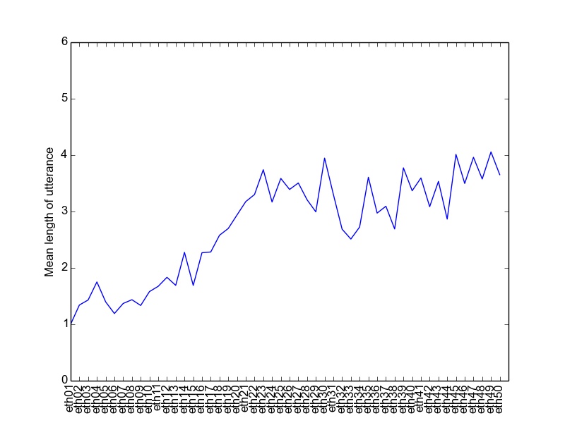
Once your plot looks right, save it as a PDF file, so you can create and compare plots across a few different children. What general trends do you see in the plots and why? Why are the plots so jagged? Suppose we wanted to use this data to directly compare the language development of the different children, i.e., whether one child is acquiring language faster than another. What information is missing from the plots you just made that would be needed in order to do this analysis?
Going Further
Have a go at some or all of the following. You may need to do some legwork to look up how to use the functions or techniques that are mentioned. Tasks 1-3 are less challenging from a programming perspective but are still good for getting you to think about the data some more. Task 4 may require a bit more programming but should also be accessible to beginners.
- Compute type/token ratios for the mothers and children in the corpus. (The type/token ratio is simply the number of unique word types divided by the number of word tokens, where in this case we would like you to compute the ratio for each mother and each child separately.) Do you see any consistent patterns? How would you illustrate or describe these patterns effectively to someone else?
- Generalize get_mlus to take a second argument that is a string. The new version should compute MLU for lines beginning with that string (e.g., you should be able to compute the MLU for MOT instead of CHI). Use Matplotlib's subplot function to plot the MLU of MOT and CHI from the same set of files in a single plot. Do you see the same trends in the MOT and CHI data? Discuss why or why not.
- Further improve the tokenization in get_word_counts so that the word counts you are collecting more accurately reflect "real" words.
- The information needed to make a fair comparison between children's language development is already in the files we gave you. Write some new code that generates MLU plots using this information, and see what you can conclude about the development of each child.
- Rewrite get_mlus without using for loops by instead using list comprehension. (This exercise is mainly intended for students who are experienced programmers but new to Python.)
- Download the Manchester corpus from CHILDES, which contains morphological annotations, and see if you can compute MLU based on the number of morphemes per utterance instead of the number of words per utterance. (Warning: you will likely run into various unanticipated issues in processing the data, this is par for the course in NLP)