MLPR w5b - Machine Learning and Pattern Recognition

$$ \newcommand{\I}{\mathbb{I}} \newcommand{\N}{\mathcal{N}} \newcommand{\bb}{\mathbf{b}} \newcommand{\bff}{\mathbf{f}} \newcommand{\bh}{\mathbf{h}} \newcommand{\bnu}{{\boldsymbol{\nu}}} \newcommand{\bu}{\mathbf{u}} \newcommand{\bx}{\mathbf{x}} \newcommand{\g}{\,|\,} \newcommand{\te}{\!=\!} \newcommand{\ttimes}{\!\times\!} $$

Autoencoders and Principal Components Analysis (PCA)

One of the purposes of machine learning is to automatically learn how to use data, without writing code by hand. When we started the course with linear regression, we saw that we could represent complicated functions if we hand-engineered features (or basis functions). Those functions can then be turned into “neural networks”, where — given enough labelled data — we can learn the features that are useful for classification automatically.

For some data science tasks the amount of labelled data is small. In these situations it is useful to have pre-existing basis functions that were fitted as part of solving some other task. We can then fit a linear regression model on top of these basis functions. Or perhaps use the basis functions to initialize a neural network, and only train for a short time.

The basis functions could come from fitting another supervised task. For example, neural networks trained on the large ImageNet dataset are often used to initialize the training of image recognition models for tasks with only a few labels. We may also wish to use completely unlabelled data, such as relevant but unannotated images, text or other data related to our task.

Autoencoders

Autoencoders solve an “unsupervised” task: find a representation of feature vectors, without any labels. This representation might be useful for other tasks. An autoencoder is a neural network representing a vector-valued function, which when fitted well, approximately returns its input: \[ \bff(\bx) \approx \bx. \] If we were allowed to set up the network arbitrarily, this function is easy to represent. For example with a single “weight matrix”: \[ \bff(\bx) = W\bx, \quad \text{with}~W=\I,~\text{the identity}. \] Constraints are required to find an interesting representation that might be useful.

Dimensionality reduction: One possible constraint is to form a “bottleneck”. We use a neural network with a narrow hidden layer with $K\ll D$ units: \[\begin{aligned} \bh &= g^{(1)}(W^{(1)}\bx + \bb^{(1)})\\ \bff &= g^{(2)}(W^{(2)}\bh + \bb^{(2)}), \end{aligned}\] where $W^{(1)}$ is a $K\ttimes D$ weight matrix, and the $g$’s are element-wise functions. If the function output manages to closely match its inputs, then we have a good lossy compressor. The network can compress $D$ numbers down into $K$ numbers, and then decodes them again, approximately reconstructing the original input.

One application of dimensionality reduction is visualization. When $K\te2$ we can plot our transformed data as a 2-dimensional scatter-plot.

When an autoencoder works well, the transformed values $\bh$ contain most of the information from the original input. We should therefore be able to use these transformed vectors as input to a classifier instead of our original data. It might then be possible to fit a classifier on smaller inputs using less labelled data. Transforming our data with no additional input from the outside world can’t add information to our vectors, an observation known as the “data processing inequality”.

Denoising and sparse autoencoders: Fitting an autoencoder with a high-dimensional hidden layer gives features that are easier to separate with a linear classifier.¹ A regularization strategy that enables setting $K\!\ge\!D$ is the denoising autoencoder: randomly set some of the features in the input to zero, but try to reconstruct the original uncorrupted vector. Then if $K\te D$ the best strategy is no longer for $W^{(1)}$ to be the identity matrix. The hidden units should represent common conjunctions of multiple input features, so that missing features can be reconstructed. Alternatively, sparse autoencoders only allow a small fraction of the $K$ hidden units to take on non-zero values. That limitation forces the network to represent the input vector as a linear combination of a small number of different “sources”. A large number, $K$, of different sources are possible, but only a few can be used for each example.

Principal Components Analysis (PCA)

When a linear autoencoder is used with the square loss function, then Principal Components Analysis (PCA) reduces the data in an equivalent way with two advantages. 1) Unlike the neural network approach, the fitted solution is unique and can be found using standard linear algebra operations. 2) The solutions for different $K$ are nested, for a given datapoint, the feature $h_1$ is the same in the solutions for all $K$, $h_2$ is the same for all $K\!\ge\!2$, and so on.

In this note, PCA reduces the dimensionality of an $N\ttimes D$ data matrix $X$, by multiplying it by a $D\ttimes K$ matrix $V$. To keep the maths simpler, we will assume for the rest of this note that the $N$ feature vectors are distributed around the origin, the dataset has been centred to have zero mean. That means that the average row in $X$ is the $D$-dimensional zero vector, in other words, that the average of the $N$ numbers in any column of $X$ is zero. We centre the data to have this property before doing anything else.

We compute the covariance matrix of the points. As we’re assuming $X$ is zero-mean, the covariance is $\Sigma = \frac{1}{N}X^\top X$. Recalling the material on multivariate Gaussians, the covariance can be used to describe an ellipsoidal ball that summarizes how the data is spread in space.²

Some axes of the ellipsoid are often very short, and the data is “squashed” into a ball that only significantly extends in some directions. The eigenvectors of the covariance matrix point along the axes of the ellipsoid, and the longest axes are the eigenvectors with the largest eigenvalues. (You can take this statement on trust, or work through Q4b of tutorial 2 again, from which you might see it.)

PCA measures the position of a data-point along the most elongated axes of the ellipsoid by setting the columns of the transformation matrix $V$ to the $K$ eigenvectors of the covariance matrix associated with the largest $K$ eigenvalues. Often (for zero mean data) we take eigenvectors of $X^\top X$, dropping the factor of $1/N$ in the covariance, which doesn’t change the directions of the eigenvectors.

% Find top K principal directions:
[V, E] = eig(X'*X);
[E,id] = sort(diag(E),1,'descend');
V = V(:, id(1:K));  % DxK

% Transform down to K-dims:
X_kdim = X*V;  % NxK

% Transform back to D-dims:
X_proj = X_kdim * V';  % NxD

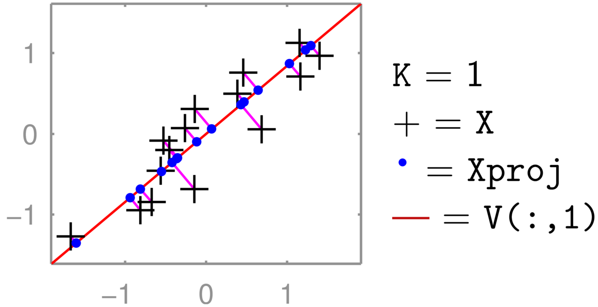
The two-dimensional coordinates of the $+$’s are reduced to one number, giving relative positions along the line that they have been projected onto (the principal component). Transforming back up to two dimensions gives the coordinates of the $\bullet$’s in the full 2-dimensional space. These projected points $XVV^\top$ are constrained to lie along a one-dimensional line. (See also the related discussion in the pre-test.) The position along the second principal axis has been lost.

The eigenvectors of a covariance matrix are orthogonal, so if all the dimensions are kept, that is $K\te D$, then $VV^\top = \I$, and no information is lost.

We can replace a feature vector $\bx$ with a transformation $A\bx$ in any model. The transformation $A$ could even be generated at random (no fitting, so no risk of overfitting!). Alternatively the transformation could be seen as $K\ttimes D$ extra parameters, and fitted as part of the model (like in a neural network). PCA is a way to fit a sensible transformation, but without fitting (and possibly overfitting) to a specific task.

PCA Examples

PCA is widely used, across many different types of data. It can give a quick first visualization of a dataset, or reduce the number of dimensions of a data matrix if overfitting or computational cost is a concern.

An example where we expect data to be largely controlled by a few numbers is body shape. The location of a point on a triangular mesh representing a human body is strongly constrained by the surrounding mesh-points, and could be accurately predicted with linear regression. PCA describes the principal ways in which variables can jointly change when moving away from the mean object.³ The principal components are often interpretable, and can be animated. Starting at a mean body mesh, one can move along each of the principal components, showing taller/shorter people, and then thinner/fatter people. The later principal components will correspond to more subtle, less interpretable combinations of features that covary.

A striking PCA visualization was obtained by reducing the dimensionality of $\approx 200,000$ features of people’s DNA to two dimensions (Novembre et al., 2008).⁴ The coordinates along the two principal axes closely correspond to a map of Europe showing where the people came from(!). The people were carefully chosen.

As is often the case with useful algorithms, we can choose how to put our data into them, and solve different tasks with the same code. Given an $N\ttimes D$ matrix, we can run PCA to visualize the $N$ rows. Or we can transpose the matrix and instead visualize the $D$ columns. As an example, I took a binary $S\ttimes C$ matrix $M$ relating students and courses. $M_{sc} \te 1$, if student $s$ was taking course $c$. In terms of these features, each course is a length-$S$ vector, or each student is a length-$C$ vector. We can reduce either of these sets of vectors to 2-dimensions and visualize them.

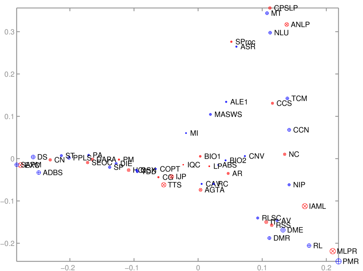
One axis (roughly) goes from computer-based applications of Informatics, through theory to broader applications. The other goes from cognitive/language applications down to machine learning. The algorithm had no labels, just which courses are taken together.

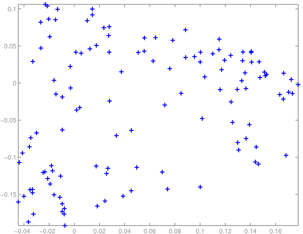
A scatter plot of students was less interpretable. I didn’t find obvious groups corresponding to the MSc specialisms offered in Informatics:

Finally, PCA doesn’t always work well. One of the papers that helped convince people that it was feasible to fit deep neural networks showed impressive results with non-linear deep autoencoders in cases where PCA worked poorly: Reducing the dimensionality of data with neural networks, Hinton and Salakhutdinov (2006). Science, Vol. 313. no. 5786, pp504–507, 28 July 2006. Available from http://www.cs.utoronto.ca/~hinton/papers.html

PCA and SVD

The truncated SVD view of PCA reflects the symmetry noted in the MSc course data example above: we can find a low-dimensional vector representing either the rows or columns of a matrix. SVD finds both at once.

Singular Value Decomposition (SVD) is a standard technique, available in most linear algebra packages. It factors a $N\ttimes D$ matrix into a product of three matrices, \[ X \approx U S V^\top, \] where $U$ has size $N\ttimes K$, $S$ is a diagonal $K\ttimes K$ matrix, and $V^\top$ has size $K\ttimes D$. The $V$ matrix is the same as before, its columns (or the rows of $V^\top$) contain eigenvectors of $X^\top X$. The columns of $U$ contain eigenvectors of $XX^\top$. The rows of $U$ give a $K$-dimensional embedding of the rows of $X$. The columns of $V^\top$ (or the rows of $V$) give a $K$-dimensional embedding of the columns of $X$.

% PCA via SVD, for zero-mean NxD matrix X
[U, S, V] = svd(X, 0);
U = U(:, 1:K); % NxK "datapoints" transformed into K-dims
S = S(1:K, 1:K);
V = V(:, 1:K); % DxK "features" transformed into K-dims
X_kdim = U*S;
X_proj = U*S*V';

A truncated SVD is known to be the best low-rank approximation of a matrix (as measured by square error). PCA is the linear dimensionality reduction method that minimizes the least squares error of the distortion when projecting onto a $K$-dimensional subspace within the original space: $X\approx XVV^\top$.

Probabilistic versions of PCA

The simplest probabilistic model of $D$-dimensional feature vectors $\bx$ that lie on a low-dimensional manifold, is to assume they’re Gaussian. The model assumes that a $K$-dimensional Gaussian variable was generated, $\bnu \sim \N(\mathbf{0},\I_K)$, and then transformed up into $D$-dimensions, $\bx = W\bnu$, where $W$ is a $D\ttimes K$ matrix. Under this model, $\bx \sim \N(\mathbf{0}, WW^\top)$. The covariance is low rank, rank $K$, because it only has $K$ independent rows or columns. By the construction, all vectors $\bx$ generated from this model will lie exactly on a linear subspace of dimension $K$.

A Gaussian with low-rank covariance isn’t able to explain real-world data, which won’t lie exactly on a linear subspace. Specifically the likelihood of such a model will be zero if any data-points lie outside the $K$-dimensional subspace. We can explain such deviations by assuming that spherical noise was added to the points from the model of the previous paragraph: $\bx \sim \N(\mathbf{0}, WW^\top + \sigma^2\I)$. This is the probabilistic PCA (PPCA) model. In the limit as $\sigma^2\rightarrow 0$ the low-dimensional explanations of the data will be the same as PCA. But a more sensible model will result by setting non-zero $\sigma^2$. PPCA is a special case of probabilistic Factor Analysis, which sets the noise to be an arbitrary diagonal covariance matrix.

Test your understanding

You will use this material on Q2 and Q3 of Tutorial 5, and briefly in the second assignment.

I train an auto-encoder on a large collection of varied images. You have a small collection of labelled images for a specialized application. Describe how and why my auto-encoder might be useful in building a classifier for your application.

Show from a definition of covariance that an element of the empirical covariance matrix $\Sigma_{ij}$ is given by $\big(\frac{1}{N}X^\top X\big)_{ij}$ for an $N\ttimes D$ design matrix $X$ that has been centred.

What choices would you consider if you were creating an autoencoder to model binary feature vectors?

What you need to know

I’m not going to ask you to prove things about eigenvectors, or the relationships between eigendecompositions and SVD, or other deep technical details relating to PCA on the exam.

You should know how PCA can be done, because it’s useful. You should also be able to discuss why it may be better or worse than other dimensionality reduction or feature extraction methods you’re asked to consider. Multivariate Gaussians come up a lot in this course, so thinking about PPCA and Factor Analysis may be useful. Again you don’t need to memorize equations, but you could be given the details and then asked about them, just as with other Gaussian models we will cover.

PCA and autoencoders find representations of your original input features. It may be easier to represent and/or learn a function based on features pre-processed with PCA or an autoencoder. However, these are operations done entirely inside your computer, after gathering data. As a reminder, you cannot “add information” about the world by processing your data, on the contrary, you can only lose information.