Computer Science Large Practical

Computer Science
Large Practical

Introduction

Paul Patras

Housekeeping

One lecture per week

When: Fridays, 12:10–13:00.

Coursework accounts for 100% of your mark.
Please ask questions at any time.
Ask offline questions on Piazza first – self-enrol here.
Office hours: Thursdays @ 10:00 in IF-2.03 (if you cannot make it and want to meet, email ppatras@inf.ed.ac.uk).

Restrictions

CSLP only available to third-year undergraduate students.
Not available to visiting UG, UG4, and MSc students.
UG3 students should choose at most one large practical, as allowed by their degree regulations.
- On some degrees (typically combined Hons) you can do the System Design Project instead/additionally.
See Degree Programme Tables (DPT) in the Degree Regulations and Programmes of Study (DRPS) for clarifications.

About this course

So far most of your practicals have been small exercises.
This practical is larger and less rigidly defined than previous course works.
The CSLP tries to prepare you for
- The System Design Project (in the second semester);
- The Individual Project (in fourth year).

Requirements

There is:
- a set of requirements (rather than a specification);
- a design element to the course; and
- more scope for creativity.
Requirements are more realistic than most coursework,
But still a little contrived in order to allow for grading.

How much time should I spend?

CSLP is now a 20 credit course.
200 hours, all in Semester 1, of which
8 hours lectures;
4 hours programme level learning and teaching
(office hours, PT meetings, training, etc.);
188 hours individual practical work.

How much time is that really?

12.5 weeks remaining in semester 1 (Weeks 2 to 14).
15 * 12.5 = 187.5 hours.
You can think of it as 15 hours/week in the first semester.
This could be just over 2 hours/day including weekends.
You could work 7.5 hours in a single day, twice a week
- for example work two days between 9:00-17:30, with an hour for lunch.

Managing your time

You may not want to arrange your work on the LP as two days where you do nothing else, but 2 days/week all semester is the amount of work you should do for CSLP.

You should not have other deadlines overlap Weeks 11-13 as your are expected to concentrate on large practicals then.

Plan wisely to avoid unpleasant surprises!

Deadlines

Part 1
- Deadline: Friday 7th October, 2016 at 16:00.
- Part 1 is zero-weighted: it is just for feedback.
Part 2
- Deadline: Friday 11th November, 2016 at 16:00.
- Part 2 is worth 50% of the marks.
Part 3
- Deadline: Wednesday 21st December, 2016 at 16:00.
- Part 3 is worth 50% of the marks.

Scheduling work

It is not necessary to keep working on the project right up to the deadline.
For example, if you are travelling home for Christmas you might wish to finish the project early.
In this case ensure that you start the project early.
The coursework submission is electronic (commit through Bitbucket) so it is possible to submit remotely,
- But you must make sure that your code works as expected on DiCE.

Extensions

Do not ask me for an extension as I cannot grant any.
The correct place is the ITO who will pass this on to the year organiser (Christophe Dubach).
See the policy on late coursework submission first.

The Computer Science Large Practical

The CSLP Requirement

Create a command-line application in a programming language of your choice (as long as it compiles and runs on DiCE).
The purpose of the application is to implement a stochastic, discrete-event, discrete time simulator
- (I will come back to these terms).
This will simulate the bin collection process in a “smart” city, with bin locations, capacities, etc. given as input.

The CSLP Requirement (C'tnd)

The output will be the sequence of events that have been simulated, as well as some summary statistics.
Input and output formats, and several other requirements are specified in the coursework handout.
It is your responsibility to read the requirements carefully.

Why Simulators?

Stochastic simulation is an important tool in physics, medicine, computer networking, logistics, etc.
Particularly useful to understand complicated processes.
Can save time, money, effort and even lives.
Allow running inexpensive experiments of exceptional circumstances that might otherwise be infeasible.
However, the simulator must have an appropriate model for the real system under investigation, to produce meaningful results.

Example: preventing Internet outages

Source: Internet Census –World map of 24 hour relative average utilization of IPv4 addresses.

Two years ago CBC news reported that in the U.S. Verizon dumped 15,000 Internet destinations for ~10 minutes.

Preventing Internet outages

Global Internet routing table has passed 512K routes.
Older routers have limited size routing tables; when these fill up, new routes are discarded.
Large portions of the Internet become unreachable, thus online businesses are loosing money.
Upgrading equipment is expensive and takes time; workarounds are being proposed.
Ensuring the proposed solutions will work is not trivial.

Preventing Internet Outages

Testing patches in live networks poses the risk of further disruption.
Waiting for the next surge is not acceptable.
Forwarding all traffic for new routes through a default interface has serious implications on routing costs.
With simulation it is possible to generate synthetic traffic and test patches without disrupting the network.

Why Simulate Bin Collection?

Waste management is a major operation in many cities.
Part of ongoing smart cities initiatives, bins are being equipped with occupancy sensors to improve scheduling and route planning for lorries.
Limitations of current periodic collection strategies:
- Lorries make unnecessary frequent trips and sometimes take lengthy routes → increased operation cost and pollution.
- User daily demand varies and could cause overflows before scheduled collection → increased health hazards and cleaning costs.

Why Simulate Bin Collection?

With simulation we can investigate the impact of different service intervals and bin occupancy thresholds used to trigger scheduling.
In this practical we will evaluate waste collection efficiency in terms of volume collected per service, percentage of overflows, etc.
- small thresholds → longer trips, but cleaner streets;
- large thresholds → cost efficient, but risk of overflows.

Your Simulator

Your simulator will be a command-line application.
It will accept an input text file with the description of the serviced areas and a set of global parameters.
It should output information about occurring events.
The strict formats for both input and output are described in the coursework handout.
You will also need to produce summary statistics that you will later analyse.

Bash Scripts

To allow for automated testing and give you the opportunity to choose the programming language you are most familiar with, you will be given two skeleton Bash scripts, which you need to modify.


   $ ./compile.sh

will be used to compile your code. The choice of compilation method is yours (as long as it works on DiCE).


   $ ./simulate.sh input_file_name [OPTIONS]

will be used to run your simulator with one (or more) command line argument(s).

Simulation Algorithm

The underlying simulation algorithm is fairly simple:


WHILE {time ≤ max time}
   determine the events that will occur after the current state
   delay ← choose a delay based on the nearest event
   time ← time + delay
   modify the state of the system based on the current event
ENDWHILE

Simulation Algorithm


WHILE {time ≤ max time}
    ...
    delay ← choose a delay based on the nearest event
    ...
ENDWHILE

Some events are deterministic, some occur with delays that follow an Erlang-k distribution.
I'll explain this in more details, but for now this is effectively the distribution of the sum of $k$ independent exponential variables with mean $\mu = 1/\lambda$, where $\lambda$ is the rate and given.

Components of the Simulation

Input - Global parameters

lorry volume,
maximum lorry load,
bin service duration,
bin volume,
rate and shape of the distribution of bag disposal events,
rubbish bag volume,
minimum and maximum bag weight limits,
number of areas.

Components of the Simulation

Input

Area description and dynamic parameters:
1. Collection frequency;
2. Bin occupancy threshold;
3. Number of bins;
4. Matrix representation of roads layout.

Components of the Simulation

Users

At any bin, users dispose of waste bags at time intervals that follow an Erlang-k distribution (rate & shape given).
Bags of fixed volume (in cubic meters), given as input.
Bag weight (in kg) is a random value, uniformly distributed between a lower and an upper bound.

Components of the Simulation

Bins & Lorries

Community bins have a fixed capacity expressed in m³;
no weight constraints.
Bins have occupancy sensors and consider occupancy thresholds used to trigger collection.
Fixed service time (in minutes) required to empty a bin, irrespective of its occupancy; service at depot 5x longer.
Lorries have fixed capacity in terms of volume and weight.
Lorries are scheduled periodically at fixed intervals.

Components of the Simulation

Service areas

We consider a directed graph representation of the bin locations and the distances between them.
The graph is given as an input in matrix form.
The distances between any two locations in minutes.

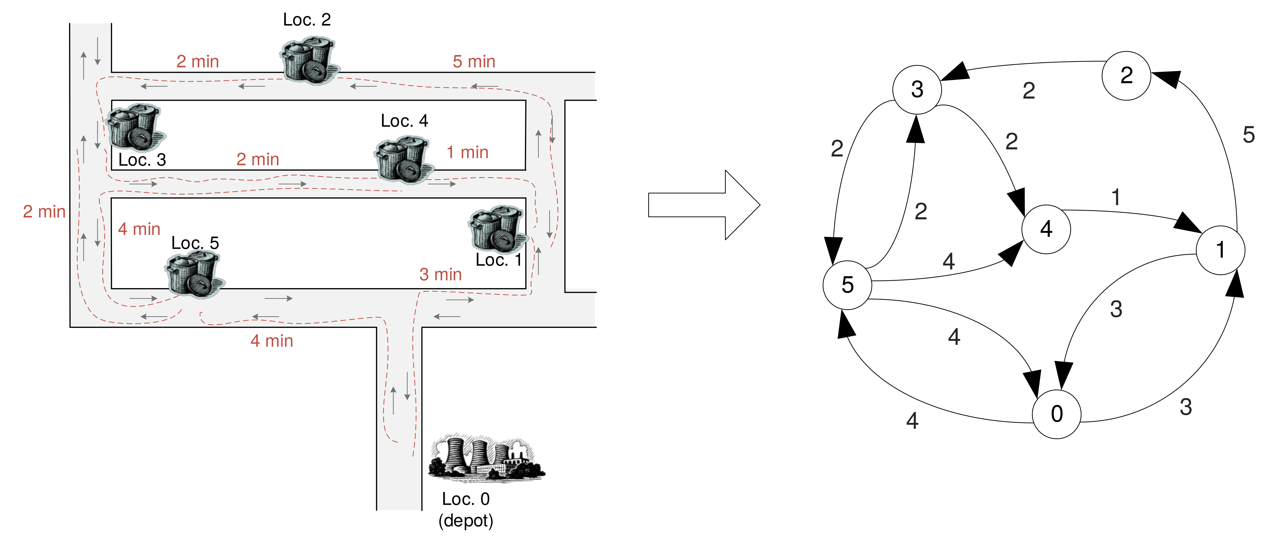
Example

Matrix representation


# Road layout and distances between bin locations (in minutes)
roadsLayout
 0  3 -1 -1 -1  4 
 3  0  5 -1 -1 -1
-1 -1  0  2 -1 -1
-1 -1 -1  0  2  2
-1  1 -1 -1  0 -1
 4 -1 -1  2  4  0

Components of the Simulation

Route planning

At every schedule, occupancy thresholds used to decide which bins need to be serviced.
All routes are circular, i.e. they must start and end at the origin (the depot).
Goal: compute optimal routes that visit all bins requiring service and minimum costs.
How you achieve this task is your design choice.
Exploring different heuristics is appropriate.

Components of the Simulation

Events

Your simulator will produce a sequence of events
- bag disposed of;
- bin load/contents volume changed;
- bin occupancy threshold exceeded;
- bin overflowed;
- lorry arrived at/left location;
- lorry load/contents volume changed.

Components of the Simulation

Events

Your simulator will output a sequence of events in the following format:


‹time› -> ‹event› ‹details›

Read the handout for full specification of output format.
Remember your code will be automatically tested, thus you need to strictly follow the output specification.
Some output could be valid in the sense that it is formatted correctly, but may be invalid for semantic reasons.

Getting Started

For this project you will use the git source control system to manage your code.
Create a Bitbucket account with your university email address and fork the CSLP-16-17 repository.
Simple instructions on how to do this in the handout.
If you haven't done this already, do this today!
It only takes a few minutes.
Keep your repository private, but do give the marker and me permissions to access that.

Code Sharing

This is an individual practical so code sharing is not allowed. Even if you are not the one benefiting.
It is somewhat likely that in the future you will be unable to publicly share the code you produce for your employer.
We will perform similarity checks and report any possible cases of academic misconduct. Don't risk it!
Start early, ask questions.

Important!

Your code will be subject to automated testing.
Strictly abiding to the input/output specification and command line formatting is mandatory.
Your code may be functional, but you will lose points if it fails on automated tests.
This is something you should expect with the evaluation of commercial products as well.
Your code will be automatically tested every week and you will be able to track your progress through an online scoreboard (details over the next days).

Assessment

Part 1, is just for feedback. You only need to submit a proposal document.
For part 2, you must have a program that compiles and runs without errors, and:
- Performs parsing and validation of input;
- Generates and schedules disposal events;
- Produces correctly formatted output;
- Is accompanied by tests scripts;
- Is appropriately structured and commented;

Assessment

For part 3, must have a fully functional simulator that:
- Performs route planning;
- Produces correct summary statistics;
- Supports experimentation;
- Is tested and optimised;
- Has evidence of appropriate source control usage;
Also produce a written report describing architecture, design choices, testing efforts, experiments performed, results obtained, insights gained.
This lecture is a summary and by no means a substitute for reading the coursework handout.

Computer Science Large Practical

Survey results

Approx. 1/5 of class responded; statistically significant?
The majority of you have substantial experience in Java, and all have at least some basic experience in Python.
Naturally, Java is the preferred choice for CSLP.

That's fine; just make sure you can work comfortably in other languages in the long run.

Nearly half of you never wrote Bash scrips

I will explain some Bash scripting concepts today; link to comprehensive tutorial on the course web page.

Survey results (II)

Almost 1/2 of respondents never used git.

Link to quick guide on course web page;
I will give a summary today.

To cover code reusability and optimisation concepts.
Graph theory: 2/3 unfamiliar with shortest path/graph traversal algorithms.
Statistics: 2/3 can only compute basic statistics (e.g. mean) or have no knowledge.

Survey results (III)

Results visualisation: major gap!

Training somewhat out of scope of these lectures, but will try to cover some basics at the end;
Guides to various tools already on course web page.

Topics you want covered:

Version control, Bash, graph theory, code optimisation, statistics → all planned;
Results plotting → time permitting;
Music (!) → Not the right course, but will try to put out a (highly subjective!) Spotify playlist for coding.

The Simulator

Definitions

In the requirements I have stated that your simulator will be a:
- stochastic,
- discrete event,
- discrete time
simulator.
Let's see what each of these terms means.

Stochasticity

A stochastic process is one whose state evolves “non-deterministically”, i.e. the next state is determined according to a probability distribution.
This means a stochastic simulator may produce slightly different results when run repeatedly with the same input.
Therefore it is appropriate to compute certain statistics to characterise the behaviour of the simulated system.
Remember, these are statistics about the model:
- You hope that the real system exhibits behaviour with similar statistics.

Discrete Events

Discrete events happen at a particular time and mark a change of state in the system.
This means discrete-event simulators do not track system dynamics continuously, i.e. an event either takes place or it does not.
There is no fine-grained time slicing of the states, i.e.
Generally a state could be encoded as an integer.
Usually it is encoded as a set of integers, possibly coded as different data types.
Discrete-event simulations run faster than continuous ones.

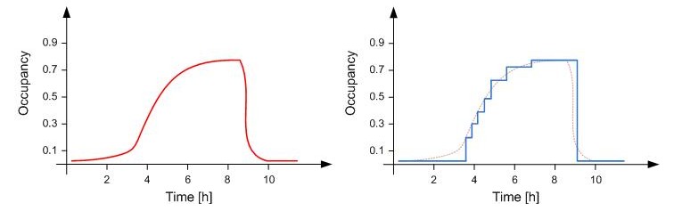
Discrete vs Continuous States

When working with discrete events, it is common to consider that states are also discrete.
Example:

Discrete Time

Discrete time simulations operate with a discrete number of points:
- Seconds, Minutes, Hours, Days, etc.
These can also be logical time points:
- Moves in a board game,
- Communications in a protocol.
Your task is to write a discrete time simulator.
Events will occur with second level granularity.

The Erlang-k Distribution

The probability distribution gives the probability of the different possible values of a random variable.
The Erlang-k distribution is the distribution of the sum of k independent exponential variables with mean $\mu = 1/\lambda$, where $\lambda$ is the rate parameter.
An exponential distribution describes the time between events in a Poisson process.

The time X between two events follows exponential distribution if the prob. that an event occurs during a certain time interval is proportional to its length.

The Erlang Distribution

Special case of Gamma distribution (Gamma allows k real)
Mean $\mu = k / \lambda$; that is if something occurs at rate $\lambda$, then we can expect to wait $k/\lambda$ time units on average to see each occurrence.
Applications: telephone traffic modelling, queuing systems, biomathematics, etc.

The Erlang Distribution

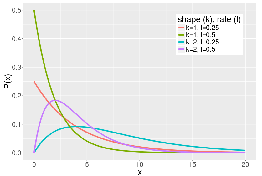
The probability density function (PDF) is given by:
Describes the relative likelihood that an event with rate $\lambda$ occurs at time $x$.

The Erlang Distribution

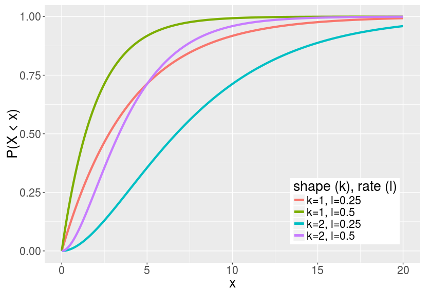
The cumulative distribution function (CDF) is given by:

The Erlang Distribution

So if something happens at a rate of 0.5 per unit of time, and the shape of the distribution is 2, then the probability that we will observe it occurring within 1 time unit is:
\[ F(1, 2, 0.5) = 1 - (e^{-0.5\times 1} + e^{-0.5\times 1}\times 0.5) = 0.09 \]

Exercise

What is the probability that a random variable $X$ is less than its expected value, if $X$ has an Erlang distribution with rate $\lambda$ and shape $k=1$?

The expected value is: $$E[X] = \frac{k}{\lambda} = \frac{1}{k}$$

Exercise

We need to compute $P(X \le E[X])$ using the distribution function:
$$P(X \le E[X]) = P(X \le 1/\lambda)$$ $$ \quad = F(x,k,\lambda)$$ $$ = 1 - e ^{-\lambda*\frac{1}{\lambda}}$$ $$ = 1 - \frac{1}{e} $$

How do we sample from a distribution?

Inverse Transform Method

Let $X$ be a RV with continuous and increasing distribution function $F$. Denote the inverse by $F ^{−1}$.
Let $U$ be a random variable uniformly distributed on the unit interval (0, 1).
Then $X$ can be generated by $X = F^{−1}(U)$.

Sampling from an Erlang distribution

If we use an Erlang CDF for $F$, then we effectively sample from that distribution by

$$X \approx \sum_{i=1}^k -\frac{1}{\lambda}\ln(U_i) = -\frac{1}{\lambda}\ln\prod_{i=1}^k U_i$$

Drawing unformly distributed numbers

You will probably do this in Java


  import java.util.Random;

  ...

  Random r = new Random();   // Uses time in ms as seed

  ...
  
  double d = r.nextDouble(); // draws between 0 (inclusive!) 
			     // and 1 (exclusive)

Remember you will need to feed that into a logarithm.

If using other languages, careful how generator is seeded.

Writing Bash Scripts

What's Bash

Command line interface for working with Unix-type systems (default on Linux, Mac OS).
You can work interactively, i.e. write commands one at the time to the prompt, press ENTER ...
or write scripts that execute multiple commands for you → great if you want to schedule jobs, test code, parse files.
A script is nothing but a text file where you write a sequence of system commands.

Bash Scripting

Make sure you made the script executable, e.g.


   $ editor test.sh
   $ chmod +x test.sh

Bash scripts typically start with a line
```
  #!/bin/bash
  
```
to let the system know this is a Bash script (you may alternatively work in Perl or others).

Bash scripting

Scripts work pretty much like any other program, so can take arguments; you can easily check how many were given, or display them


  ... 
  echo "Number of arguments $#"

  if [[ $# > 0 ]] ; then
   echo "First argument $1"
  else
   echo "No arguments given"
  fi

Running produces:


  $ ./test.sh param
  Number of arguments: 1

Bash scripting

A couple of things happened in this example:

echo used to print to standard output;
the $ character preceded arguments (same for variables);
$# used to retrieve the number of arguments passed;
Used an if statement to check if number of arguments was no-zero; it wasn't so $1 was identifying the first;
IMPORTANT: Careful about the spaces; Bash is very picky when it comes to writing conditionals;
To launch a script put ./ before script name.

Scripting your application

Your program must take as argument an input script (this is THE input containing all the simulation parameters; not to be confused with the Bash script!)
The Bash script will take the name of the input and pass it down to your executable file.
This in turn must be able to handle command line arguments.
Bash script snippet:
```
  ...
  java Simulator $1
  
```

Scripting your application

Java code:


class Simulator{
  public static void main(String args[]){
    System.out.println("Arguments passed:");
    for (String s: args) {
      System.out.println(s);
    }
  }
}

Executing script:


  $ ./test.sh basic_input
  Arguments passed:
  basic_input

Design choices

There are a few things you need to decide whether to implement inside the Bash script or inside your Java/C/Python/other code.
This includes checking if arguments have been passed, displaying usage information, checking if the file exists when a file is expected as argument, etc.
This is entirely your choice.
You may later write more sophisticated scripts to run experiments on multiple files through a single command.
Bash works nicely with AWK for text processing (parsing your output).

Source Code Control

For this project must git for version control and the Bitbucket platform.

This is somewhat realistic
Any project you join will likely already have some form of source code control set up which you will have to learn to use rather than any system you might already be familiar with
See the git homepage for detailed documentation.

Source Code Control

The practical is not looking for you to become an expert in git;
You will not need to be able to perform complicated branches or merges;
This is, after all, an individual practical
What is key, is that your commits are appropriate:
- Small frequent commits of single units of work;
- Clear, coherent and unique commit messages.

Getting Started

By now I assume everyone has forked the skeleton CSLP-16-17 repository and granted read permissions to the marker and me.
You can start with a simple README file to plan and document your work (use any text editor you wish).


  $ cd simulator
  $ editor README.md
  $ git add README.md
  $ git commit -m "Initial commit including a README"
  $ git push origin master

The main point

After each portion of work, commit to the repository what you have done.
Everything you have done since your last commit, is not recorded.
You can see what has changed since your last commit, with the status and diff commands:


$ git status
# On branch master
nothing to commit (working directory clean)

Staging and Committing

When you commit, you do not have to record all of your recent changes. Only changes which have been staged will be recorded
You stage those changes with the git add command.
Here a file has been modified but not staged


$ editor README.md
$ git status
# On branch master
# Changed but not updated:
#   (use "git add ‹file›..." to update what will be committed)
#   (use "git checkout -- ‹file›..." to discard changes in working directory)
#
#	modified:   README.md
#
no changes added to commit (use "git add" and/or "git commit -a")

Unrecorded and Unstaged Changes

A git diff at this point will tell you the changes made that have not been committed or staged


$ git diff
diff --git a/README.md b/README.md
index 9039fda..eb8a1a2 100644
--- a/README.md
+++ b/README.md
@@ -1 +1,2 @@
 This is a stochastic simulator.
+It is a discrete event/state, discrete time simulator.

To Add is to Stage

If you stage the modified file and then ask for the status you are told that there are staged changes waiting to be committed.
To stage the changes in a file use git add


$ git add README.md
$ git status
# On branch master
# Changes to be committed:
#   (use "git reset HEAD ‹file›..." to unstage)
#
#	modified:   README.md
#

Viewing Staged Changes

At this point git diff is empty because there are no changes that are not either committed or staged.
Adding --staged will show differences which have been staged but not committed.


$ git diff # outputs nothing
$ git diff --staged
diff --git a/README.md b/README.md
index 9039fda..eb8a1a2 100644
--- a/README.md
+++ b/README.md
@@ -1 +1,2 @@
 This is a stochastic simulator.
+It is a discrete event/state, discrete time simulator.

New Files

Creating a new file causes git to notice there is a file which is not yet tracked by the repository.
At this point it is treated equivalently to an unstaged/ uncommitted change.


$ editor mycode.mylang
$ git status
# On branch master
# Changes to be committed:
#   (use "git reset HEAD ‹file›..." to unstage)
#
#	modified:   README.md
#
# Untracked files:
#   (use "git add ‹file›..." to include in what will be committed)
#
#	mycode.mylang

New Files

git add is also used to tell git to start tracking a new file.
Once done, the creation is treated exactly as if you were modifying an existing file.
The addition of the file is now treated as a staged but uncommitted change.


$ git add mycode.mylang
# On branch master
# Changes to be committed:
#   (use "git reset HEAD ‹file›..." to unstage)
#
#	modified:   README.md
#	new file:   mycode.mylang
#

Committing

Once you have staged all the changes you wish to record, use git commit to record them.
Give a useful message to the commit.


$ git commit -m "Added more to the readme and started the implementation"
[master a3a0ed9] Added more to the readme and started the implementation
 2 files changed, 2 insertions(+), 0 deletions(-)
 create mode 100644 mycode.mylang

Pushing

Your changes are now committed to your local working copy.
You must also send those changes to the remote Bitbucket repository, otherwise the marker/I will not be able to see the updates.


   $ git push origin master

A Clean Repository Feels Good

After a commit, you can take the status, in this case there are no changes
In general though there might be some if you did not stage all of your changes


$ git status
# On branch master
nothing to commit (working directory clean)

Finally git log

The git log command lists all your commits and their messages


$ git log
commit a3a0ed90bc90e601aca8cc9736827fdd05c97f8d
Author: Name ‹author email›
Date:   Wed 28 Sep 09:15:32 BST 2016

    Added more to the readme and started the implementation

commit 22de604267645e0485afa7202dd601d7c64c857c
Author: Name ‹author email›
Date:   Wed 28 Sep 09:15:32 BST 2016

    Initial commit

Announcement

Cisco International
Internship Programme

If you have an interest in computer networks, this is an opportunity to spend 1 year (2017-18) in Silicon Valley.
Cisco covers salary, housing, travel, etc.
Applications open early October.
Deadline: 12 December, 2016 (5:00PM EST).
Priority will be given to "early" submissions.
Details available at http://myciip.com/

`git` recap

Check status since last commit:


$ git status

Stage changes/add new files:


$ git add file_name

Record changes (advisable for new units of code):


$ git commit -m "Relevant message here"

Push to remote repository (so we can see your code):


   $ git push origin master

Lists all your commits:


$ git log

Simulation Components

Service Areas & Route Planning

Service Areas

We need an abstract representation of roads layout and bin locations for the different areas.
We need to model the roads between different locations and the time required to travel these.
We need to account for the fact that some streets only allow one way traffic.

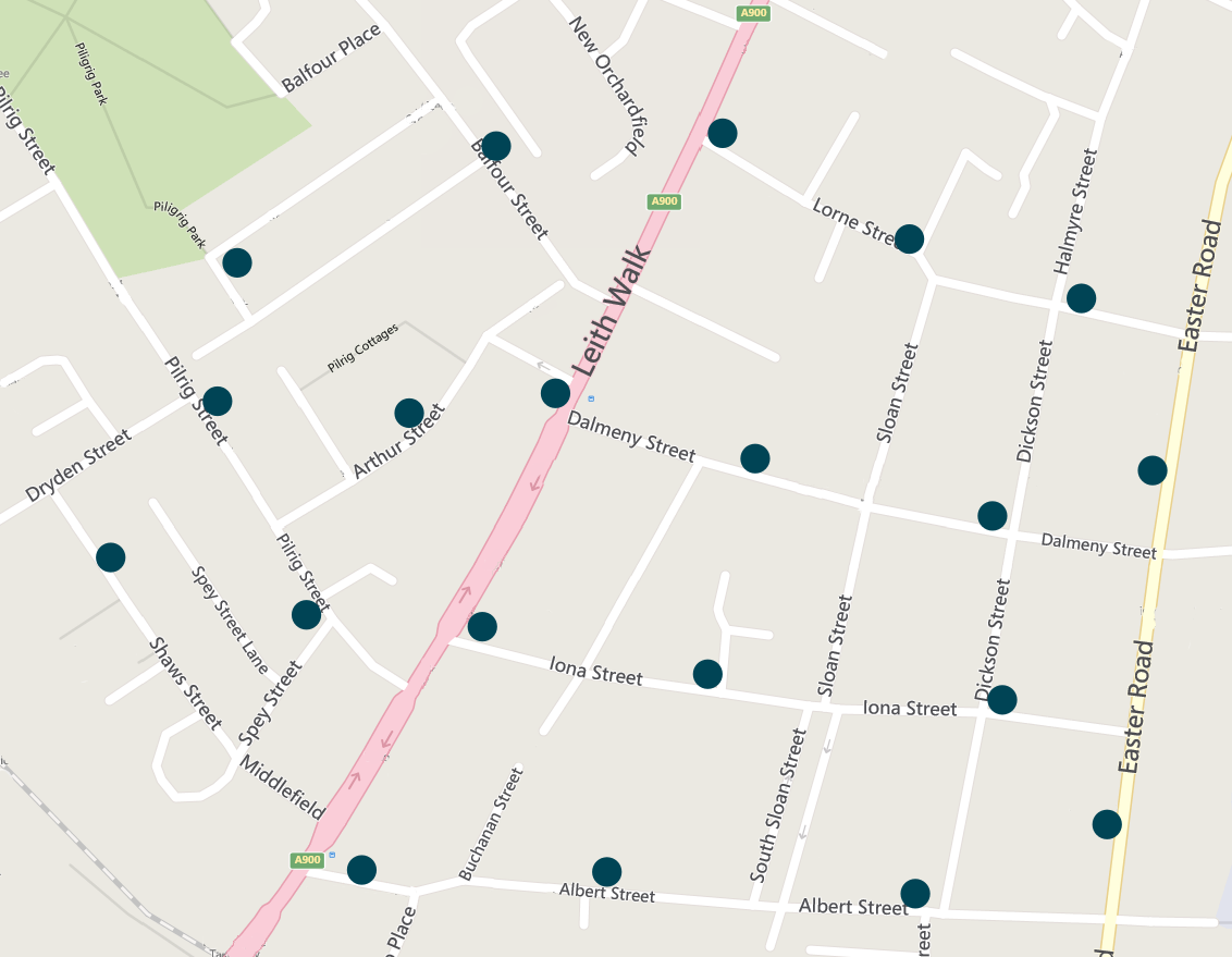
Example

Leith Walk, Edinburgh; 20 bin locations. (bing.com)

Graph representation

In mathematical terms such a collection of bin locations interconnected with street segments can be represented through a graph.
A graph G = (V,E) comprises a set of vertices V that represent objects (bin locations/depot) and E edges that connect different pairs of vertices (links/street segments).
Graphs can be directed or undirected.

Undirected Graphs

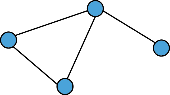
Edges have no orientation, i.e. they are unordered pairs of vertices. That is there is a symmetry relation between nodes and thus (a,b) = (b,a).

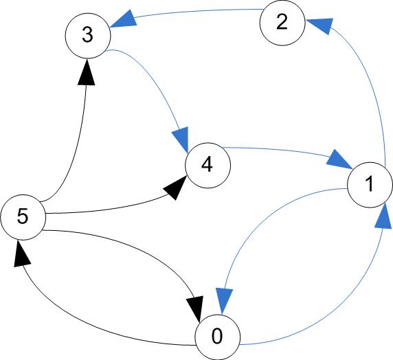
Directed Graphs

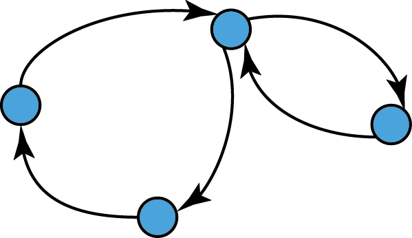
Edges have a direction associated with them and they are called arcs or directed edges.
Formally, they are ordered pairs of vertices,
i.e. (a,b) ≠ (b,a) if a ≠ b.

Graph representation in your simulators

For our simulations we will consider directed graph representations of the service areas.
This will increase complexity, but is more realistic.

Back to the example

This area...

Corresponding Graph

...can be represented by

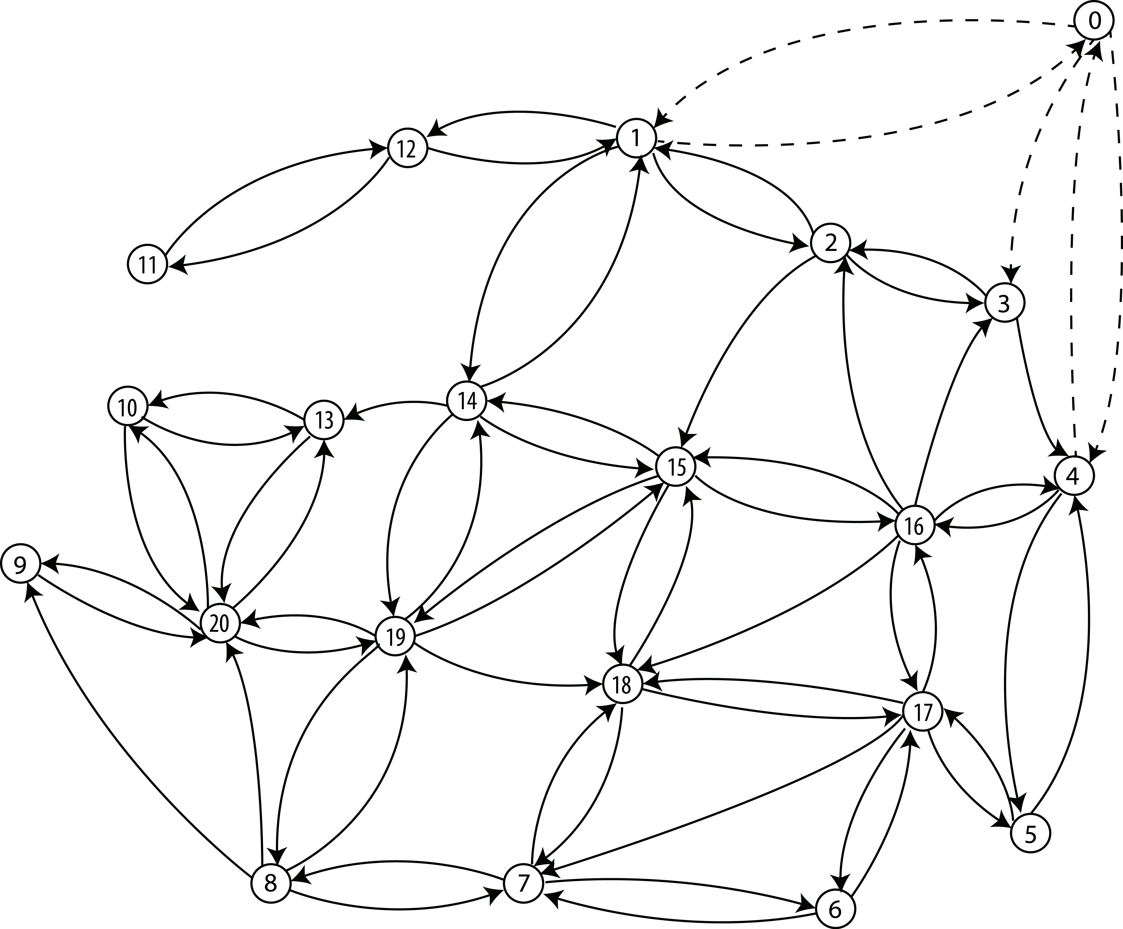
We numbered vertices & added node '0' for the depot.

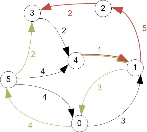
Weighted Graph

We also need to model the distances between bin locations.
We will use a weighted graph representation, where a number (weight) is associated to each arc.
In our case weights will represent the average travel duration between two locations (vertices) in one direction, expressed in minutes.

Weighted Graph

For our example, this may be

Input

For each area, graph representation of bin locations and distances between them will be given in the input script (file) in matrix form.
We will consider the lorry depot as location 0. For a service area with N locations, an N x N matrix will be specified.
The roadsLayout keyword will precede the matrix.
Where there is no arc in the graph between two vertices we will use a -1 value in the matrix.

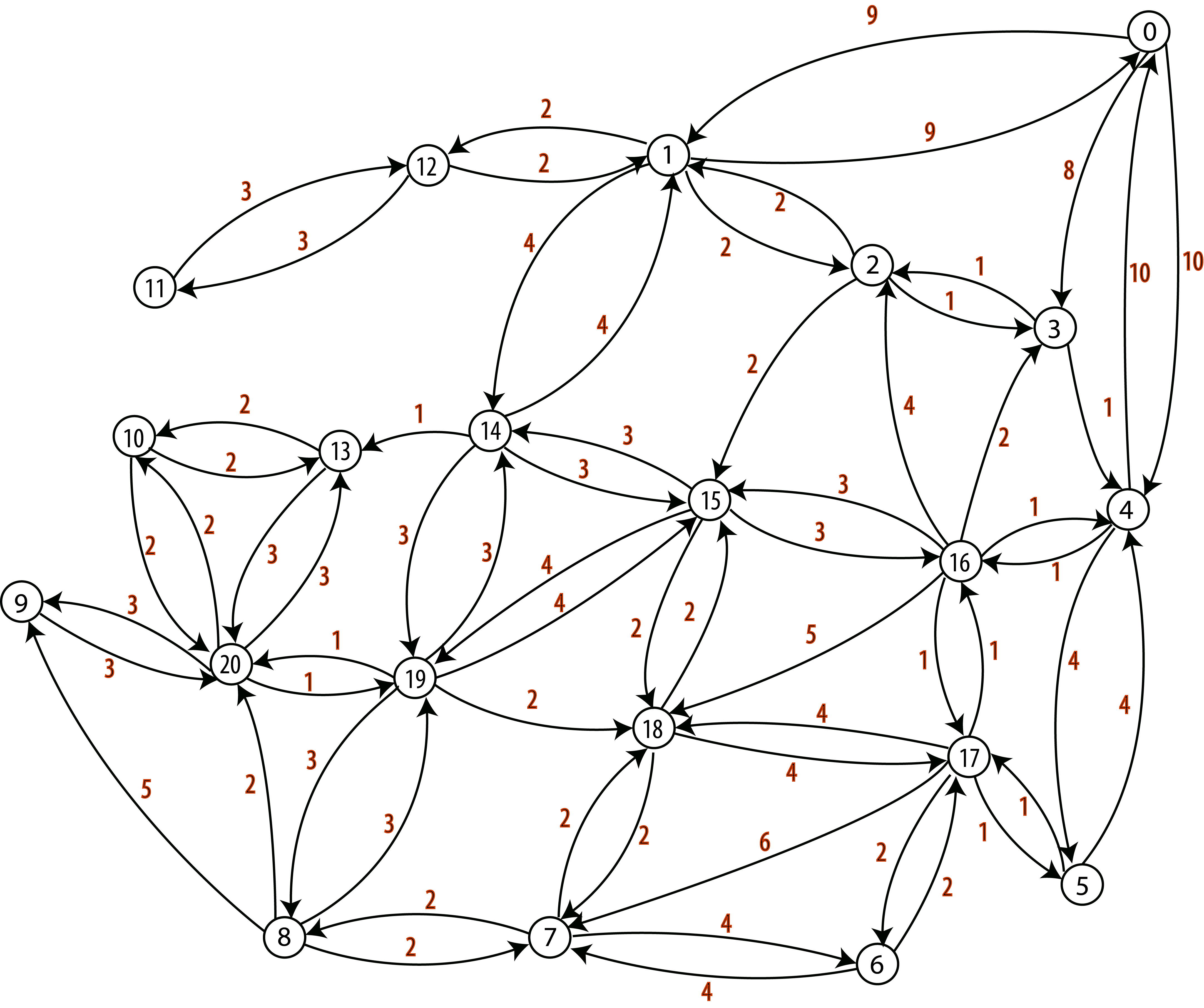
For The Previous Example


    0     1     2     3     4     5   ...   19    20
   ---------------------------------------------------
 0| 0     9    -1     8    10    -1   ...   -1    -1
 1| 9     0     2    -1    -1    -1   ...   -1    -1
 2|-1 	  2     0     1    -1    -1   ...   -1    -1
 3|-1    -1     1     0     1    -1   ...   -1    -1
 4|10    -1    -1     1     0     4   ...   -1    -1
 5|-1    -1    -1    -1     4     0   ...   -1    -1
 .| .     .     .     .     .     .          .     .
 .| .     .     .     .     .     .          .     .
 .| .     .     .     .     .     .          .     .
19|-1    -1    -1    -1    -1    -1   ...    0     1
20|-1    -1    -1    -1    -1    -1   ...    1     0

*Note that the matrix is not symmetric.

Route Planning

In each area the lorry is schedule at fixed intervals.
The occupancy thresholds are used to decide which bins need to be visited.
There are lorry weight and volume constraints that you may account for at the start when planning.
Equally, you may decide on the fly, i.e. when lorry capacity exceeded.
Naturally there are efficiency implications here. You need to chose the approach and explain why you did that.
This is not something to argue for/against. The purpose is for you to think critically about different approaches.

Route Planning

Your goal is to compute shortest routes that service all bins exceeding occupancy thresholds at the minimum cost in terms of time.
Remember all routes are circular, i.e. they begin and end at the depot.
Some bins along a route may not need service.
Thus it may be appropriate to work with an equivalent graph where vertices that do not require to be visited are isolated and equivalent arc weights are introduced.
Sometimes it may be more efficient to travel multiple times through the same location, even if the route previously serviced bins that required that.

The (More) Challenging Part

How to partition the service areas and find (almost) optimal routes that visit all vertices that require so with minimum cost?
This is entirely up to you, but I will discuss some useful aspects next.
You must justify your choice in the final report and comment appropriately the simulator code.
You may wish to implement more than one algorithm.

Useful terminology

A walk is a sequence of arcs connecting a sequence of vertices in a graph.
A directed path is a walk that does not include any vertex twice, with all arcs in the same direction.
A cycle is a path that starts & ends at the same vertex.

directed paths / cycle

Useful terminology

A trail is a walk that does not include any arc twice.
A trail may include a vertex twice, as long as it comes and leaves on different arcs.
A circuit is a trail that starts & ends at the same vertex

trail / circuit (tour)

Shortest paths

There may be multiple paths that connect two vertices in a directed graph.
In a weighted graph the shortest path between two vertices is that for which the sum of the arc costs (weights) is the smallest.

Shortest paths

There are several algorithms you can use to find the shortest paths on a given service area.
A non-exhaustive list includes

Dijkstra's algorithm (single source),
Floyd-Warshall algorithm (all pairs),
Bellman-Ford algorithm (single source).

Each of these have different complexities, which depend on the number of vertices and/or arcs.
The size and structure of the graph will impact on the execution time.

Floyd–Warshall Algorithm

A single execution finds the lengths of the shortest paths between all pairs of vertices.
The standard version does not record the sequence of vertices on each shortest path.
The reason for this is the memory cost associated with large graphs.
We will see however that paths can be reconstructed with simple modifications, without storing the end-to-end vertex sequences.

Floyd–Warshall Algorithm

Complexity is O(N³), where N is the number of vertices in the graph.

The core idea:

Consider d_i,j,k to be the shortest path from i to j obtained using intermediary vertices only from a set {1,2,...,k}.
Next, find d_i,j,k+1 (i.e. with nodes in {1,2,...k+1}).

This could be d_i,j,k+1 = d_i,j,k or
A path from vertex i to k+1 concatenated with a path from vertex k+1 to j.

Floyd–Warshall Algorithm

Then we can compute all the shortest paths recursively as

d_i,j,k+1 = min(d_i,j,k, d_i,k+1,k + d_k+1,j,k).

Initialise d_i,j,0 = w_i,j (i.e. start form arc costs).
Remember that in your case the absence of an arc between vertices is represented as a -1 value, so you will need to pay attention when you compute the minimum.

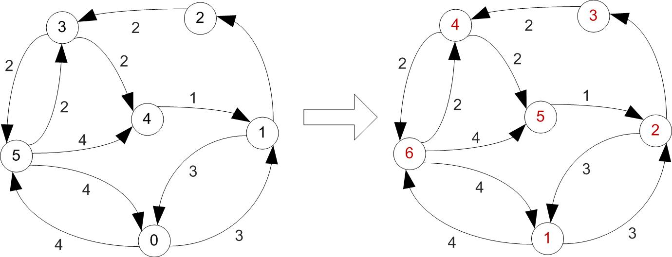
Example

First let's increase vertex indexes by one, since we were starting at 0.

Example

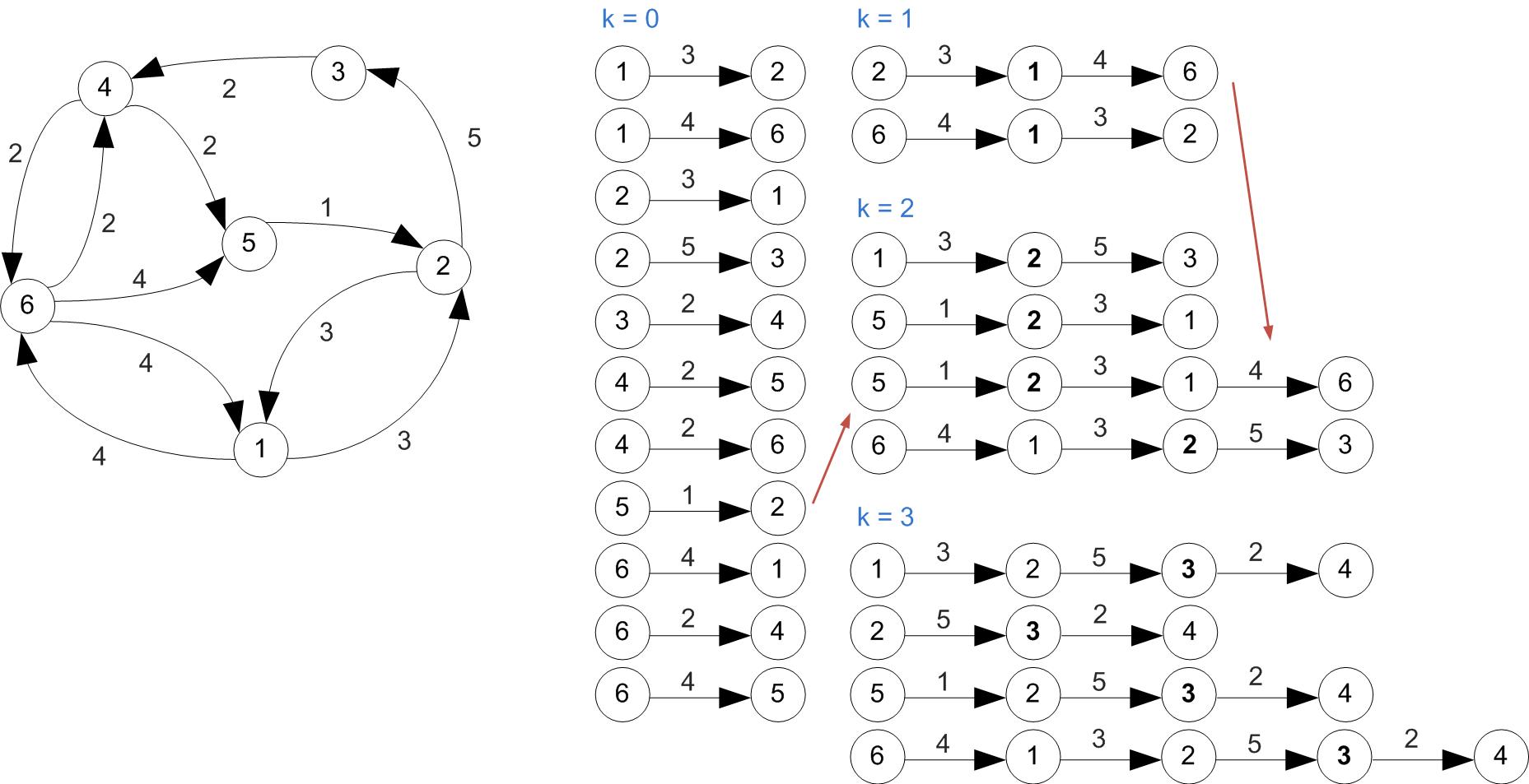
Example (Cont'd)

All shortest paths found at this step.

Pseudocode


Denote d the N × N array of shortest path lengths.
Initialise all elements in d with inf.

For i = 1 to N
   For j = 1 to N
     d[i][j] ← w[i][j]   // assign weights of existing arcs;
   
For k = 1 to N
   For i = 1 to N
       For j = 1 to N
         If d[i][j] > d[i][k] + d[k][j] 
             d[i][j] ← d[i][k] + d[k][j]
         End If

Floyd–Warshall Algorithm

This will give you the lengths of the shortest paths between each pair of vertices, but not the entire path.
You do not actually need to store all the paths, but you would want to be able to reconstruct them easily.
The standard approach is to compute the shortest path tree for each node, i.e. the spanning trees rooted at each vertex and having the minimal distance to each other node.

Pseudocode


Denote d, nh the N × N arrays of shortest path lengths and 
respectively the next hop of each vertex.

For i = 1 to N
   For j = 1 to N
     d[i][j] ← w[i][j]   // assign weights of existing arcs;
     nh[i][j] ← j
   
For k = 1 to N
   For i = 1 to N
       For j = 1 to N
         If d[i][j] > d[i][k] + d[k][j] 
             d[i][j] ← d[i][k] + d[k][j]
	     nh[i][j] ← nh[i][k]
         End If

Reconstructing the paths

To retrieve the sequence of vertices on the shortest path between nodes i and j, simply run a routine like the following.


   path ← i
   While i != j
     i ← nh[i][j]
     append i to path
   EndWhile

Finding Optimal Routes Given a Set of User Requirements

Finding shortest paths between different bin locations is only one component of route planning.
The problem you are trying to solve is a flavour of the Vehicle Routing Problem (VRP). This is a known hard problem.
Simply put, an optimal solution may not be found in polynomial time and the complexity increases significantly with the number of vertices.

Heuristic Algorithms

Heuristics work well for finding solutions to hard problems in many cases.
Solutions may not be always optimal, but good enough.
Work relatively fast.
When the number of vertices is small, a 'brute force' approach could be feasible.
Guaranteed to find a solution (if there exists one), and this will be optimal.

Clarifications

If returning to depot and having to immediately service other bins in the same schedule, should I check the occupancy status of all bins again?

No. This was not explicitly discussed in the handout, and can be debatable. For this exercise, check all bins at the beginning of a schedule, and plan according to their status even if performing multiple trips.

If visiting some bin locations on a path between two bins requiring service, should I output all that information?

No. This is useful to check your implementation is correct, but takes up memory.

Choosing Route Planning Algorithms

You have complete freedom to choose what heuristic you implement, but
make sure you document your choice and discuss its implication on system’s performance in your report.
It is likely that you will need to compute shortest paths.
Again, you can choose any algorithm for this task, e.g. Floyd-Warshall, Dijkstra, etc., but explain your choice.
You can implement multiple solutions, as some may not work for any graph or will perform poorly.
More about route planning next time.

Assignment, Part 1

Not mandatory, zero weighted (just for feedback)
Short proposal document outlining planned simulator.
You should be able to explain plans for:

Handling command line arguments;
Parsing and validation of input scripts;
Generation, scheduling, and execution of events;
Graph manipulation/route planning algorithms;
Statistics collection;
Experimentation support and results visualisation;
Code testing.

Assignment, Part 1

No code will be checked.
Have created 'doc' folder inside repository, copy 'proposal.pdf' inside, git push.


$ cd doc
$ git add proposal.pdf
$ git commit -m ’Added proposal document’
$ git push

Deadline today, 7 Oct at 16:00.

Questions?

Music

Some asked for music in the pre-course survey.

Here is a Spotify playlist you could make the soundtrack to your coding efforts. Enjoy!

Graph Traversal

Path Finding and Graph Traversal

Path finding refers to determining the shortest path between two vertices in a graph.
We discussed the Floyd–Warshall algorithm previously, but you may achieve similar results with the Dijkstra or Bellman-Ford algorithms.
Graph traversal refers to the problem of visiting a set of nodes in a graph in a certain way.
You can use depth- or breadth-first search algorithms to traverse an entire graph starting from a given "root" (source vertex).

Path Finding and Graph Traversal

Today we will discuss some heuristics for finding circuits (tours) on graphs.
We are particularly interested in finding circuits that also have minimum cost.
Remember that circuits can include the same vertex twice, but arcs only once.
You may want to perform some pre-processing on the graph to handle such restrictions.

Terminology: Hamiltonian Circuit

A Hamiltonian circuit is a path that visits every vertex exactly once and starts at ends at the same vertex
NB: Not all graphs may have a Hamiltonian circuit

Minimum Cost Hamiltonian Circuit

In a weighted graph, the minimum cost Hamiltonian circuit is that where the sum of the arc weights is the smallest.
Finding the minimum cost Hamiltonian circuit on your bin service graphs is one option for route planning.
Finding a Hamiltonian circuit can be difficult. This is a known NP-complete problem. Simply put, the problem may not be solvable in polynomial time and the complexity increases with the number of vertices.

Heuristic Algorithms

Heuristics work quite well for finding (not always optimal, but good) solutions, most of the time.
Work relatively fast.
Popular heuristics for finding minimum cost Hamiltonian circuits:

Nearest Neighbour Algorithm
Sorted Edges Algorithm

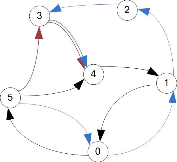
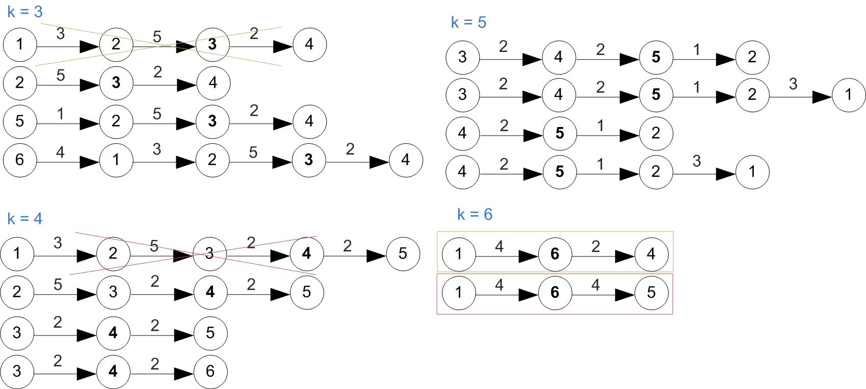
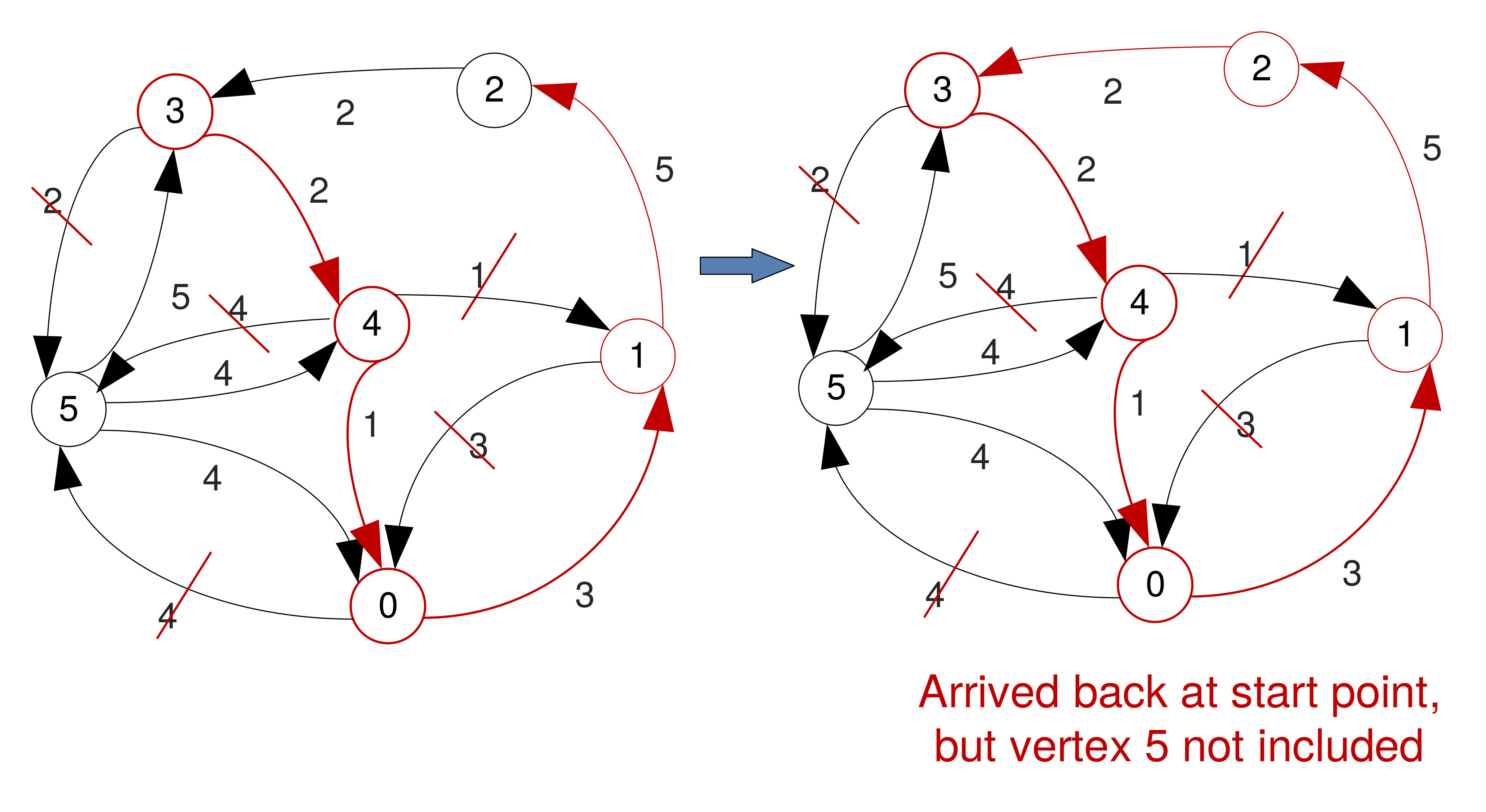
Nearest Neighbour Algorithm

Nearest Neighbour is a greedy algorithm – at every step it chooses as the next vertex the one connected to the current through the arc with the smallest weight.
Only searches locally.
Nodes already visited are ignored.
Due to its greedy nature it may not find a solution.
Finding a solution and its total cost depends on the start vertex chosen.

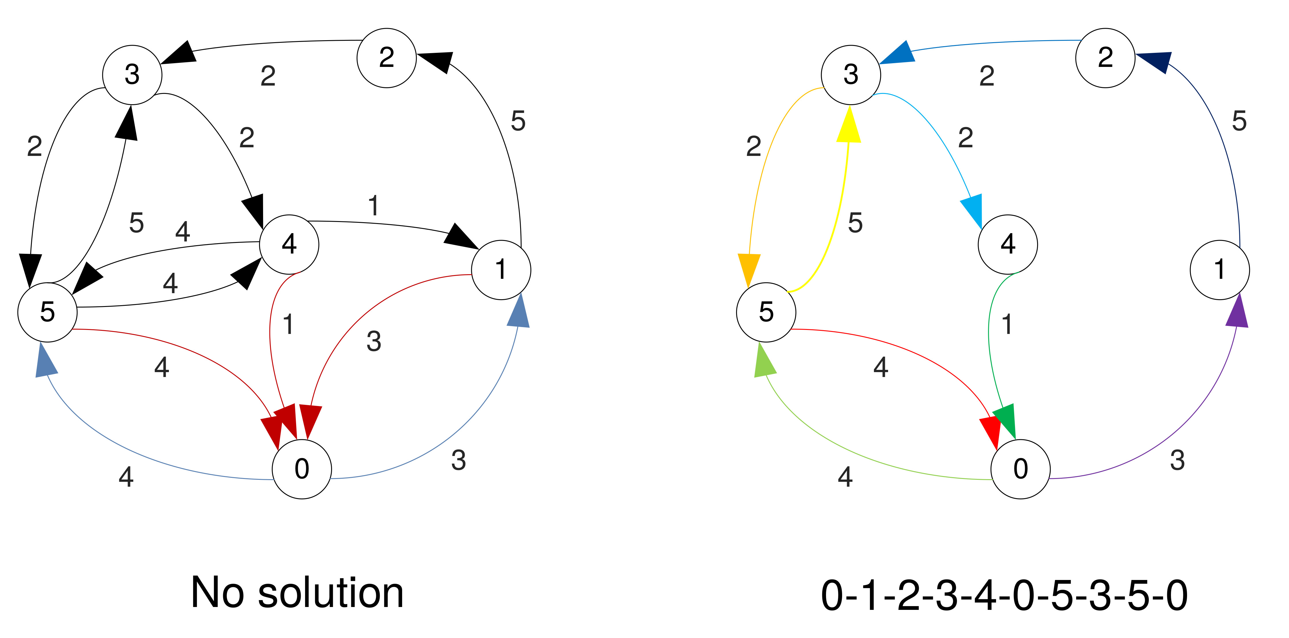
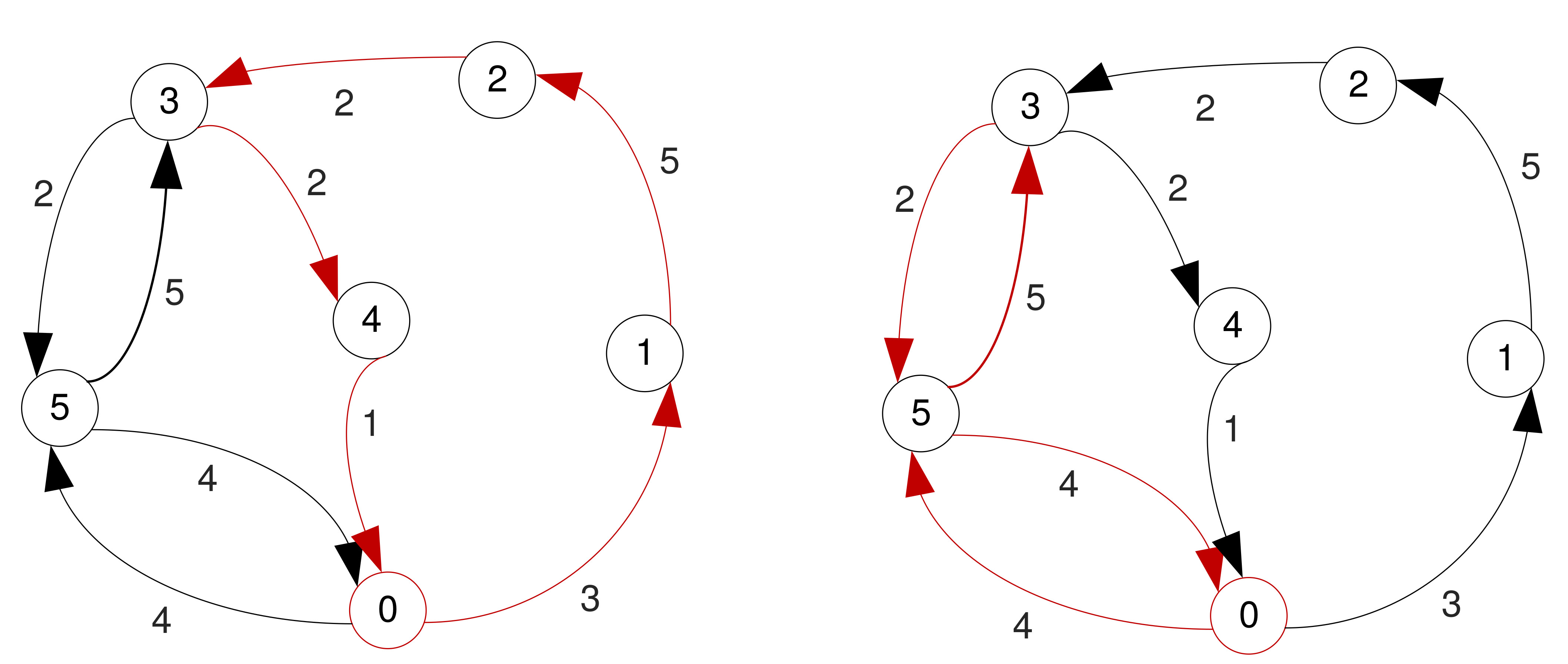
Example, starting at '3'

Example, starting at '3' (No solution)

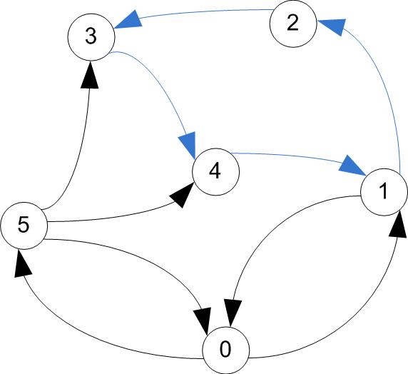
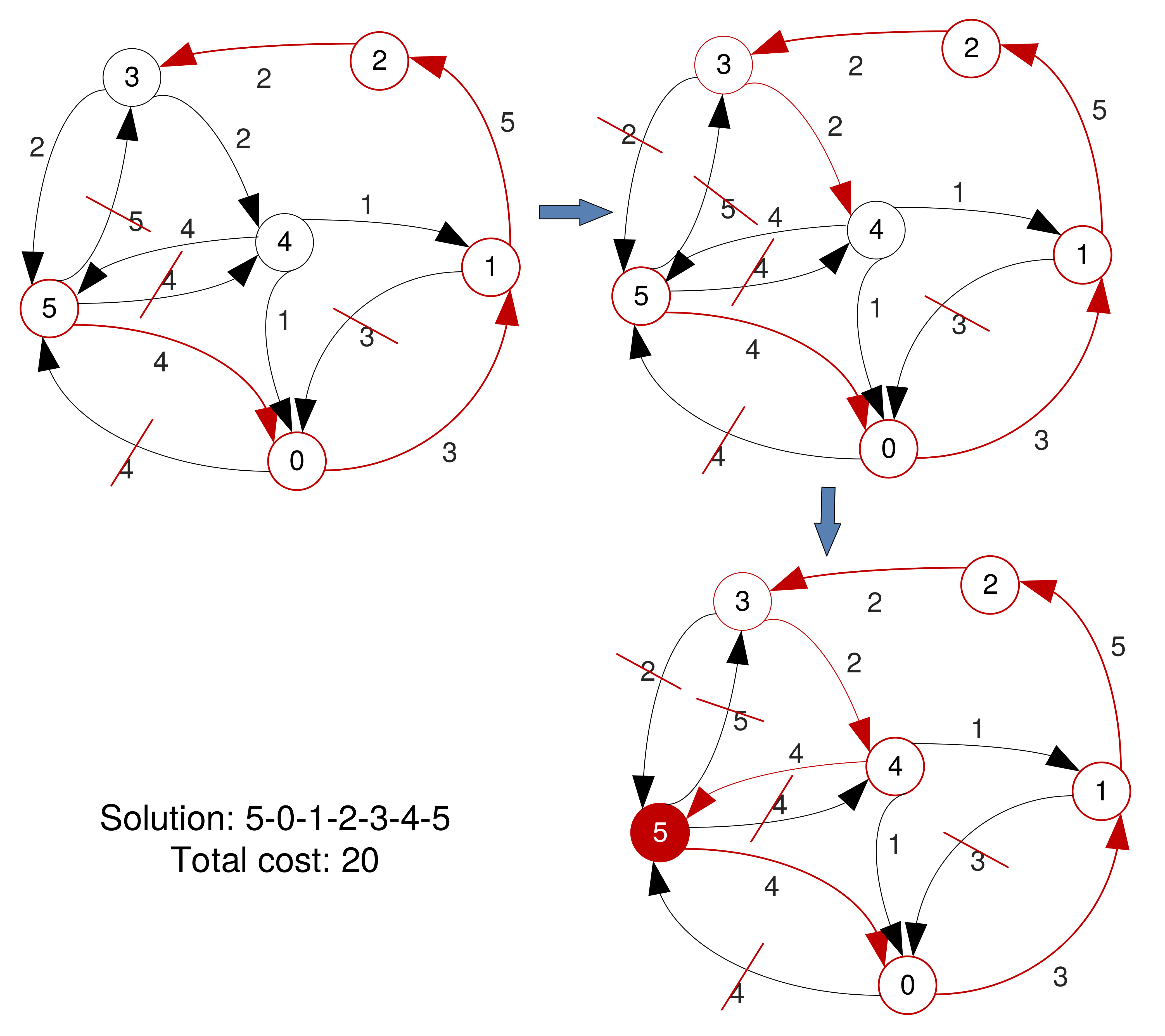
Example, starting at '5'

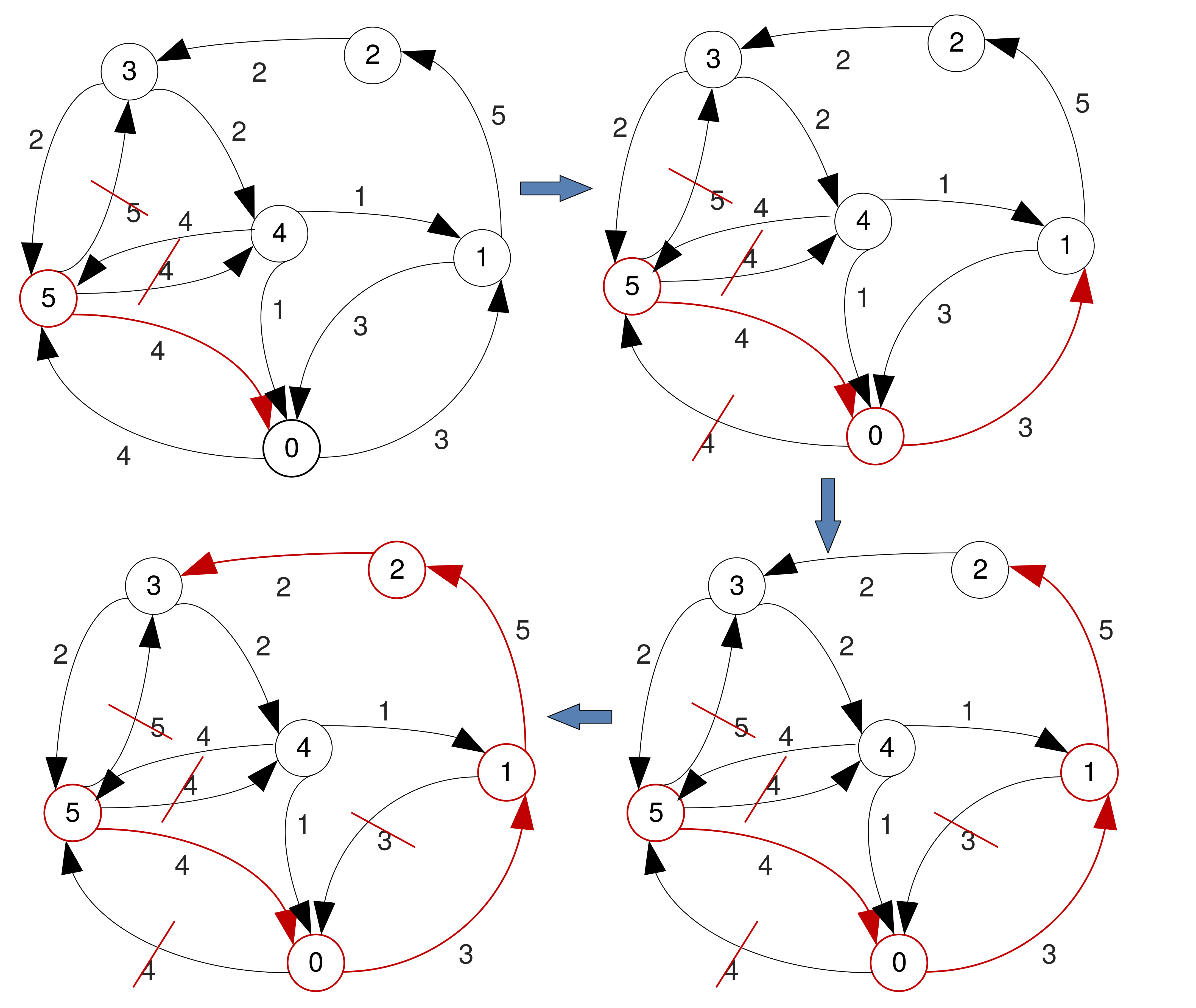
Example, starting at '5' (Cont'd)

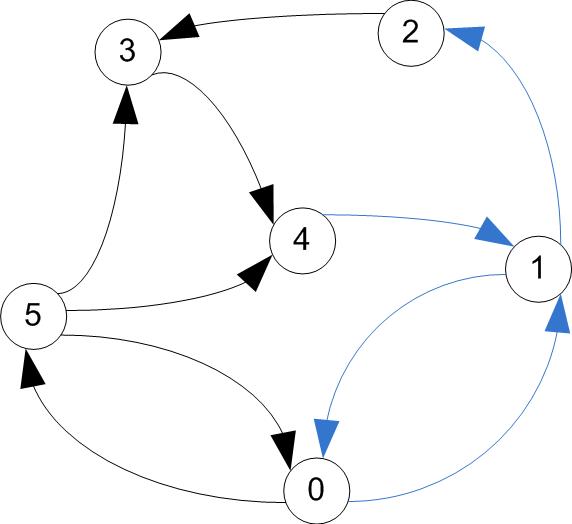
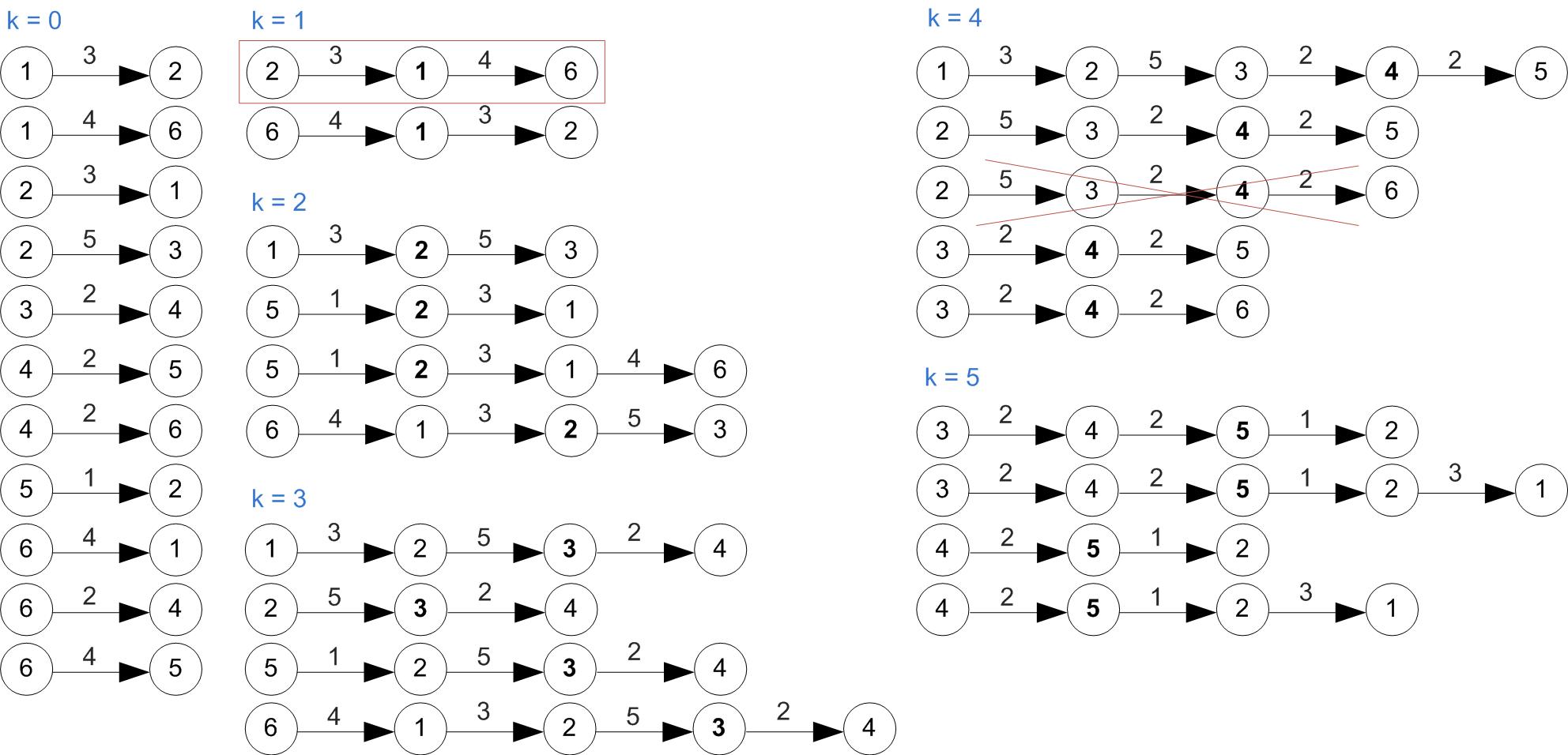
Sorted Edges Algorithm

Also greedy, but has a more global view → takes slightly more time to find a solution.
First sorts all the (directed) edges in ascending order of their weights.
Adds sorted edges one at the time, unless adding a new one leads to three arcs entering/leaving a node, or creates a circuit that does not include all vertices.
Skips the arcs that violate these rules.
Keeps adding arcs until finding a Hamiltonian circuit (or no more arcs left).
Stops when a solution is found, even if there are arcs left.

Example

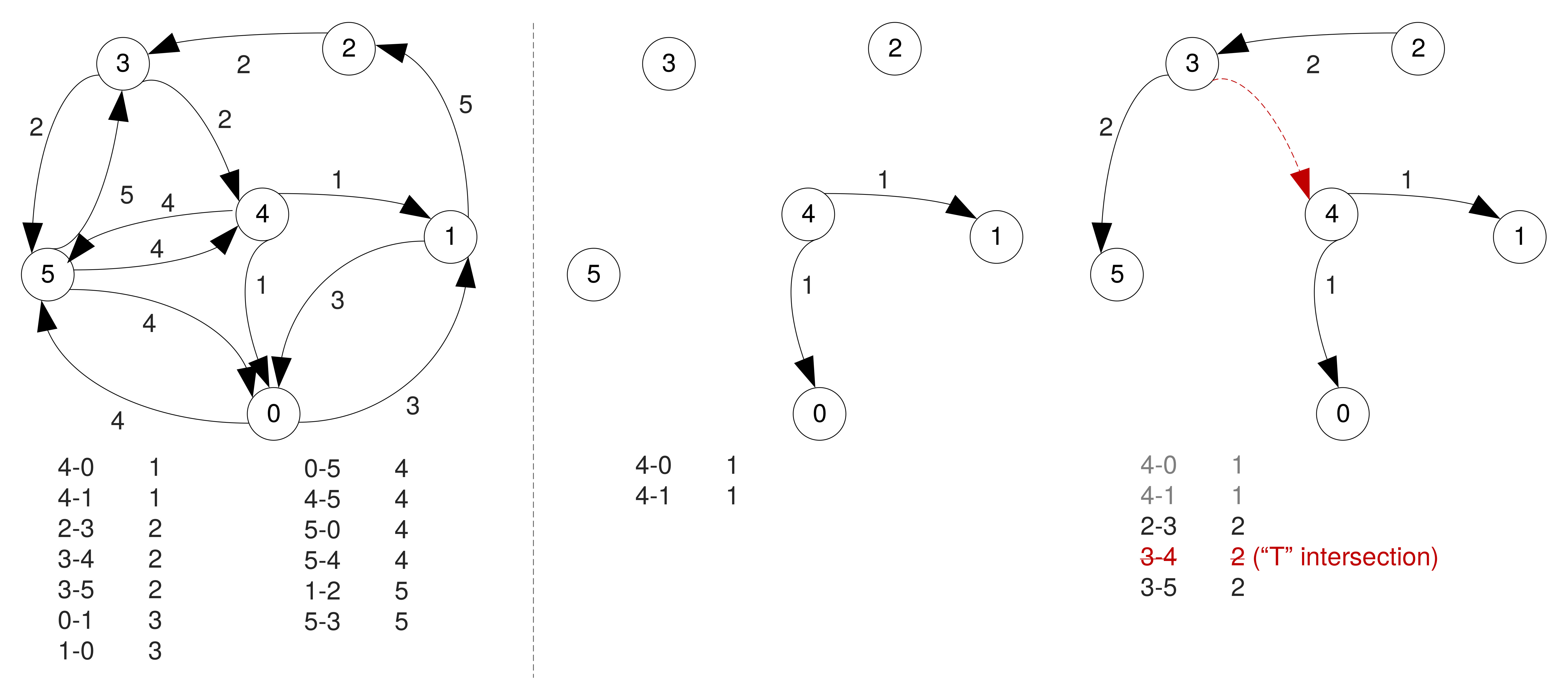
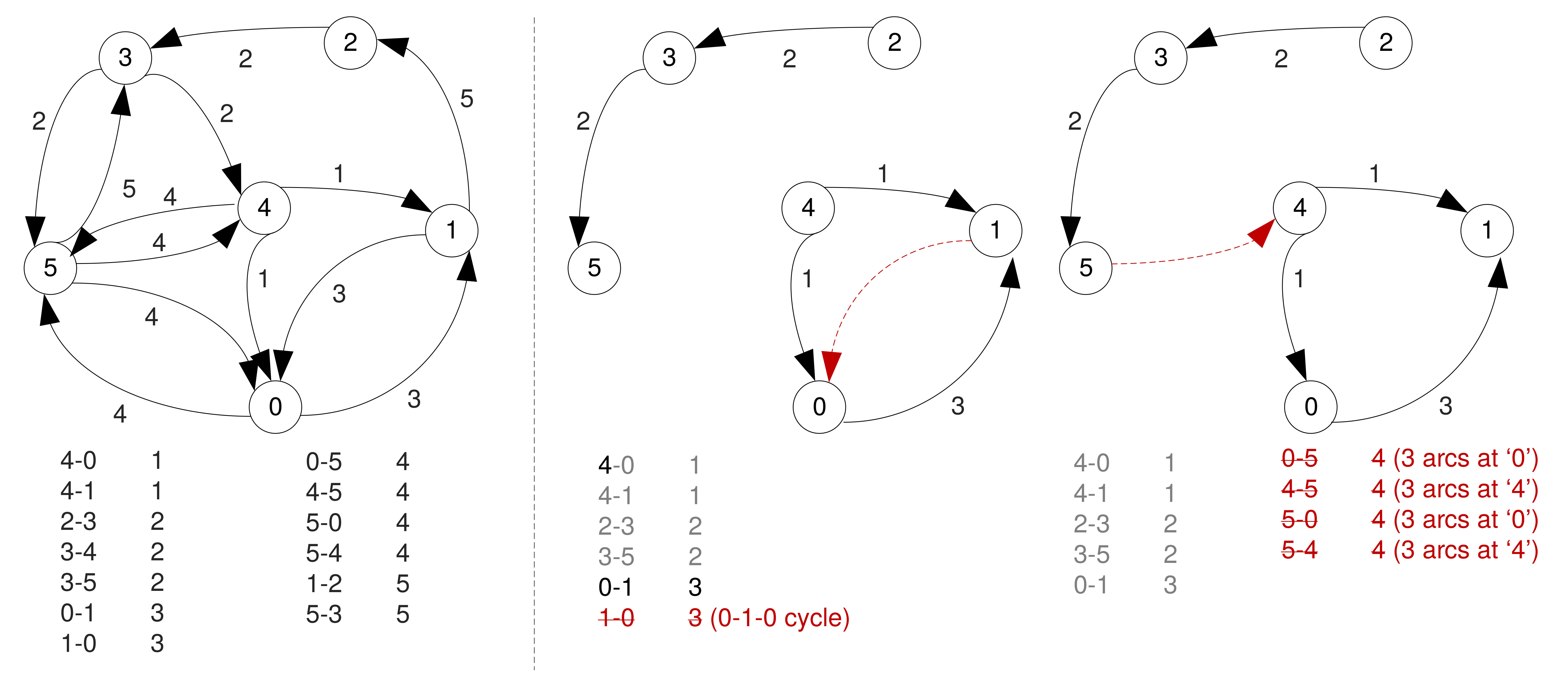
Example (Cont'd)

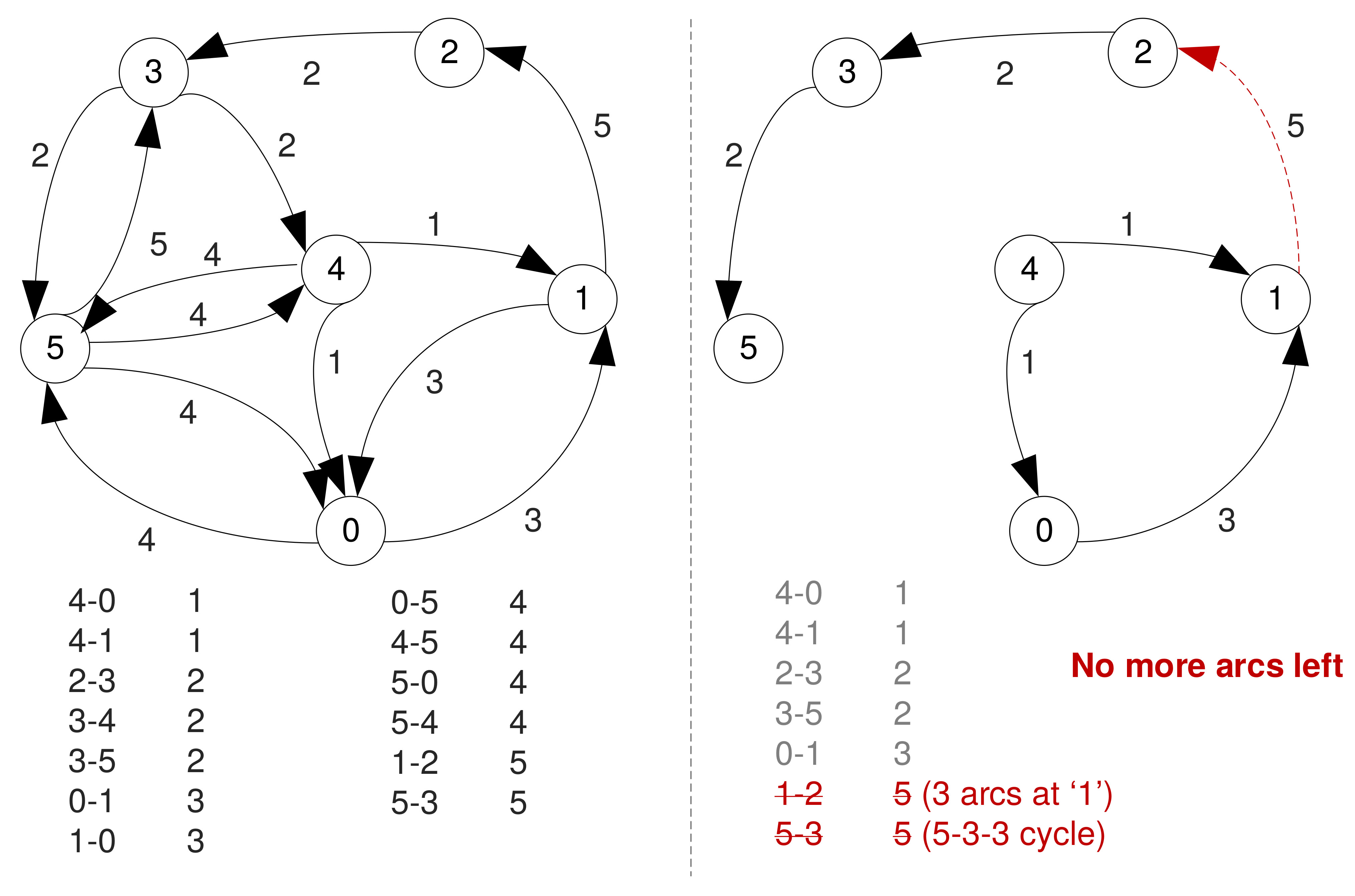
No solution found.

Brute Force Algorithm

When the number of vertices is small, a 'brute force' approach could be feasible.
Find all paths that visit all vertices once and pick the one with the lowest cost.
Guaranteed to find a solution (if there exists one), and this will be optimal.

Other approaches

A Hamiltonian circuit may not always be the path that visits all the vertices and has the lowest cost.
Sometimes visiting a node more than once can give circuits that are more cost effective.
The problem could also be seen as an instance of finding an Eulerian circuit (cycle).

Eulerian circuits

An Eulerian path visits every edge (arc) exactly once.
The idea dates back to birth of Graph Theory, when Leonhard Euler was asked to determine a path that traverses all of the 7 bridges in Koenigsberg exactly once.

Source: Nature Biotechnology

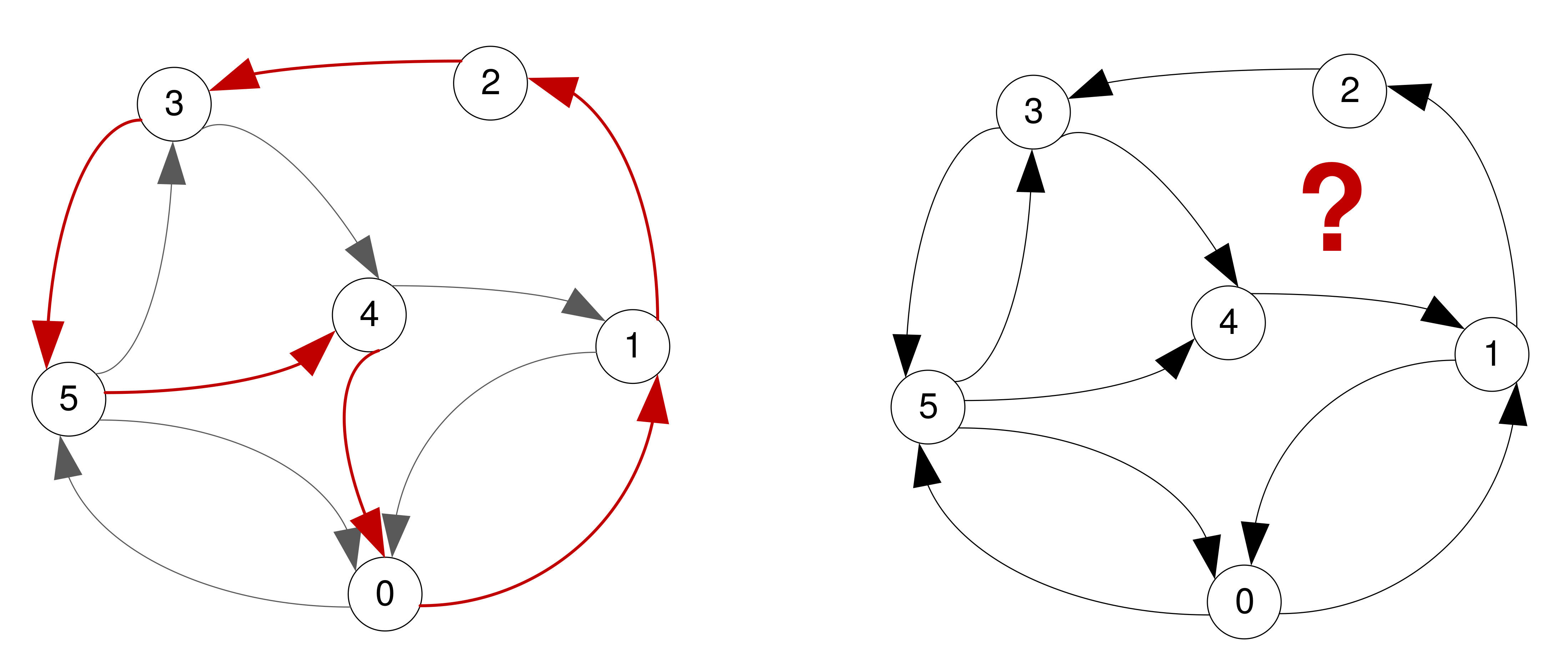
Eulerian circuits

An Eulerian circuit begins and ends at the same vertex.
Euler realised a solution to the original problem did not exist, but found conditions that a graph must fulfil to have Eulerian paths.
For your problem (directed graphs), it is important to know Eulerian circuits exist if and only if every vertex has equal in degree and out degree.

Examples

Total cost: 28

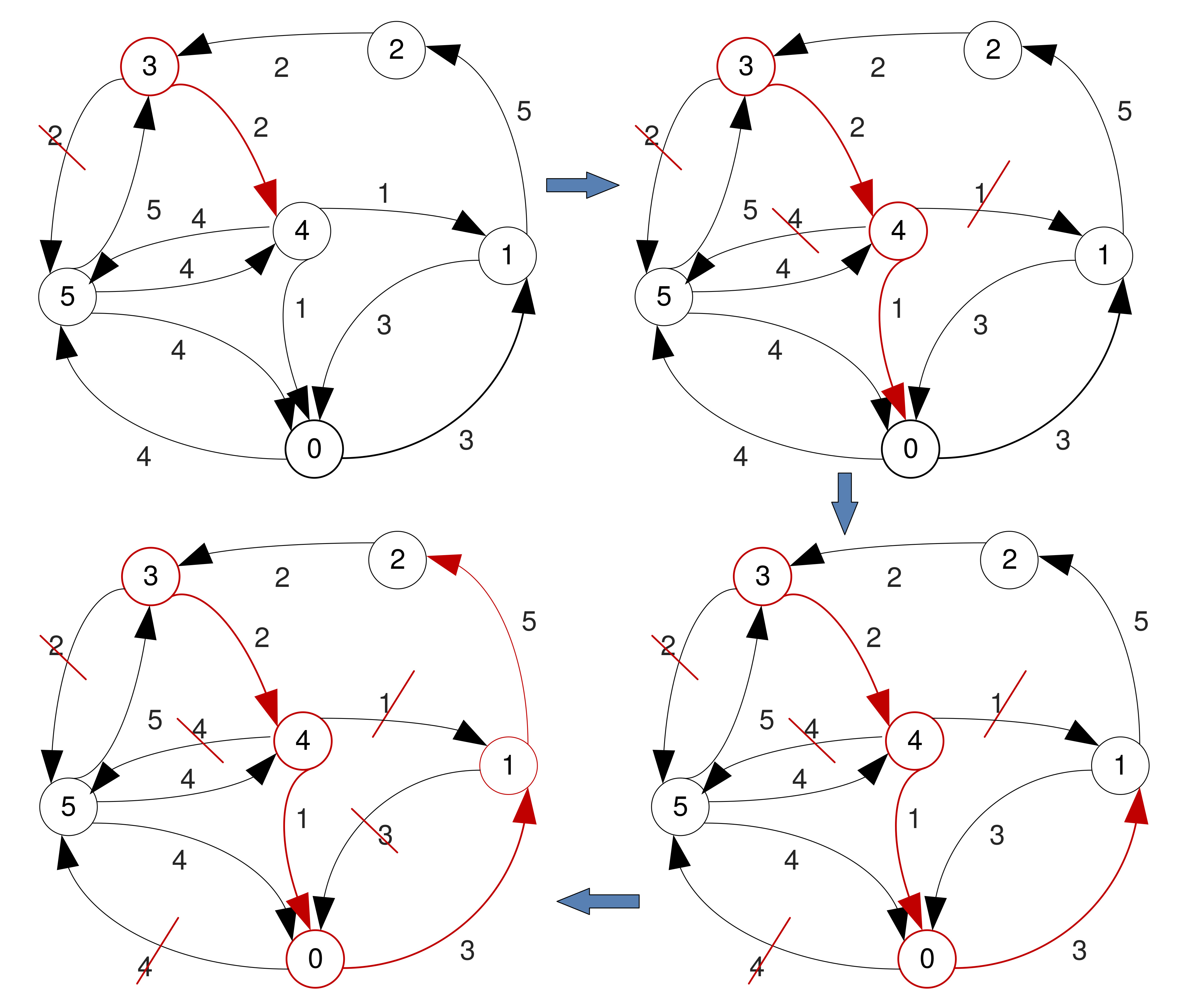
Hierholzer's algorithm

Assuming you have verified the necessary condition the graph must meet to have an Eulerian circuit,
Pick any vertex as a starting point.
Add arcs to build trail, until returning to the start. You cannot get stuck at other vertices.
If there are vertices on this tour but have adjacent arcs not included, start new trail from these.
Join the tours formed this way.

Example

The problem you are trying to solve

The graphs you will be given may not have Hamiltonian or Eulerian circuits.
Even if they do, at start of service in an area you may not need to visit ALL the bins (vertices).
It is likely you will need to do some pre-processing, e.g.

Build complete graphs starting from the original ones.
Remove some arcs.

And work only with a subset of vertices (the bins that require service).

The problem you are trying to solve

There is no BEST solution.
Depending on the graph structure/size, some may return more cost effective circuits than others.
But may also take more time.
Try to experiment with several, but aim to have at least ONE decent implementation.

Code Structuring & Coding Strategy

How to structure your work?

This is for guidance only and I will not go into great detail, to avoid seeing identically structured solutions.
Part of the practical is structuring it yourself. However, it is likely you will want at least the following components:
- A parser,
- A representation of the states of a simulation,
- The simulation algorithm,
- Something to handle output,
- Something to analyse results,
- A test suite.

Some Obvious Decisions

Do you want to parse into some abstract syntax data structure and then convert that into a representation of the initial state,
- Or could you parse directly into the representation of the initial state?
Do you wish to print out events as they occur during the simulation,
- Or record them and print them out later?
Do you wish to analyse the simulation events as the simulation proceeds,
- Or analyse the events afterwards?

Parsing

You do not necessarily need to start with the parser.
The parser produces some kind of data structure. You could instead start by hard coding your examples in your source code.
Though the parsing for this project is pretty simple.
Hence you could start with the parser, even if not complete, but remember your parser is marked at Part 2.
- Hard coding data structure instances could prove laborious,
- but doing so would ensure your simulator code is not heavily coupled with your parser code.

Software Construction

Software construction is relatively unique in the world of large projects in that it allows a great deal of back tracking.
Many other forms of projects, such as construction, event planning, and manufacturing, only allow for backtracking in the design phase.
The design phase consists of building the object virtually (on paper, on a computer) when back tracking is inexpensive.
Software projects do not produce physical artefacts, so the construction of the software is mostly the design.

Refactoring

Refactoring is the process of restructuring code while achieving exactly the same functionality, but with a better design.
This is powerful, because it allows trying out various designs, rather than guessing which one is the best.
It allows the programmer to design retrospectively once significant details are known about the problem at hand.
It allows avoiding the cost of full commitment to a particular solution which, ultimately, may fail.

More About Refactoring

Refactoring is a term which encompasses both factoring and defactoring.
Generally the principle is to make sure that code is written exactly once.
We hope for zero duplication.
However, we would also like for our code to be as simple and comprehensible as possible.

Factoring and Defactoring

We avoid duplication by writing re-usable code.
Re-usable code is generalised.
Unfortunately, this often means it is more complicated
Factoring is the process of removing common or replaceable units of code, usually in an attempt to make the code more general.
Defactoring is the opposite process specialising a unit of code usually in an attempt to make it more comprehensible.

Factoring Example


void primes(int limit){
    integer x = 2;
    while (x <= limit){
        boolean prime = true;
        for (i = 2; i < x; i++){
            if (x % 2 == 0){ prime = false; break; }
        }
        if (prime){ System.out.println(x + " is prime"); }
    }
}

A very naive but perfectly reasonable bit of code to print out a set of prime numbers up to a particular limit.

Factoring Example


void print_prime(int x){
    System.out.println(x + " is prime");
}
void primes(int limit){
    x = 2;
    while (x <= limit){
        ... // as before
        if (prime){ print_prime(x); }
    }
}

Here we have “factored out” the code to print the prime number to the screen. This may make it more readable, but the code is not more general.

Factoring Example

To make it more general we have to actually parametrise what we do with the primes once we have found them.


interface PrimeProcessor{
    void process_prime(int x);
}
class PrimePrinter implements PrimeProcessor{
    public void process_prime(int x){
        System.out.println(x + " is prime");
    }
}
void primes(int limit, PrimeProcessor p){
    x = 2;
    while (x <= limit){
        ... // as before
        if (prime){ p.process_prime(x); }
    }
}

You can now use different functions to display, store, etc. the prime numbers.

Factoring

We can go further and factor out the testing as well:


interface PrimeTester{
    boolean is_primes(int x);
}
class NaivePrimeTester implements PrimeTester{
    public boolean is_prime(int x){
        for (i = 2; i < x; i++){
            if (x % 2 == 0){ return false; }
        }
        return true;
    }
}
void primes(int limit, PrimeTester t, PrimeProcessor p){
    x = 2;
    while (x <= limit){
        if (t.is_prime(p)){ p.process_prime(x); }
    }
}

Factoring

Now that testing is factored out, it does not have to be used solely for primes.


interface IntTester{
    boolean property_holds(int x);
}
class NaivePrimeTester implements IntTester{
    public boolean property_holds(int x){
        for (i = 2; i < x; i++){
            if (x % 2 == 0){ return false; }
        }
        return true;
    }
} // Similarly for PrimeProcessor to IntProcessor
void number_seive(int limit, IntTester t, IntProcessor p){
    x = 0;
    while (x <= limit){
        if (t.property_holds(p)){ p.process_integer(x); }
    }
}

Factoring

Print the perfect numbers:


interface IntTester{
    boolean property_holds(int x);
}
class PerfectTester implements IntTester{
    public boolean property_holds(int x){
        return (sum(factors(x)) == x);
    }
} // Similarly for PerfectProcessor
void number_seive(int limit, IntTester t, IntProcessor p){
    x = 0;
    while (x <= limit){
        if (t.property_holds(p)){ p.process_integer(x); }
    }
}

Factoring

So which version do we prefer? This one:


public abstract class NumberSeive{
    abstract boolean property_holds(int x);
    abstract void process_integer(int x);
    abstract int start_number;
    void number_seive(int limit){
        x = self.start_number;
        while (x <= limit){
            if (self.property_holds(p)){ self.process_integer(x); }
        }}} // Close all the scopes
public class PrimeSeive inherits NumberSeive{
    public boolean property_holds(int x){
        for (i = 2; i < x; i++){
            if (x % 2 == 0){ return false; }
        }        return true;  }
    void process_integer(int x) { System.out.println (x + " is prime!"); }
    int start_number = 2;
}

Factoring

Or the original version?


void primes(int limit){
    integer x = 2;
    while (x <= limit){
        boolean prime = true;
        for (i = 2; i < x; i++){
            if (x % 2 == 0){ prime = false; break; }
        }
        if (prime){ System.out.println(x + " is prime"); }
    }
}

Factoring

Something in between?


LinkedList get_primes(int limit){
    int x = 2; LinkedList results = new LinkedList();
    while (x <= limit){
        boolean prime = true;
        for (i = 2; i < x; i++){
            if (x % 2 == 0){ prime = false; break; }
        }
        if (prime){ results.append(x); }
    }
}
void primes(int limit){ 
    for x in get_primes(limit){
        System.out.println(x + " is prime"); 
    }
}

Factoring

What you should factor depends on the context.
How likely am I to need more number seives?
How likely am I to do something other than print the primes?
Try to find the right re-usability/time trade-off.

Defactoring

Numbers such as the number 20 can be factored in different ways
- 2,10
- 4,5
- 2,2,5
If we have the factors 2 and 10, and realise that we want the number 4 included in the factorisation we can either:
- Try to go directly by multiplying one factor and dividing the other, or
- Defactor 2 and 10 back into 20, then divide 20 by 4.

Defactoring

Similarly, your code is factored in some way.
In order to obtain the factorisation that you desire, you may have to first defactor some of your code.
This allows you to factor down into the desired components.
This is often easier than trying to short-cut across factorisations.

Sieve of Eratosthenes

Create a list of consecutive integers from 2 to n: (2, 3, ..., n)
Initially, let p equal 2, the first prime number
Starting from p, count up in increments of p and mark each of these numbers greater than p itself in the list
- These will be multiples of p: 2p, 3p, 4p, etc.; note that some of them may have already been marked.
Find the first number greater than p in the list that is not marked
- If there was no such number, stop
- Otherwise, let p now equal this number (which is the next prime), and repeat from step 3

Sieve of Eratosthenes


void primes(int limit){
    LinkedList prime_numbers = new LinkedList();
    boolean[] is_prime = new Array(limit, true);
    for (int i = 2; i ‹ Math.sqrt(limit); i++){
        if (is_prime[i]){
            prime_numbers.append(i);
            for (j = i * i; j ‹ limit; j += i){
                is_prime[j] = false;
    }

You can probably do this via our abstract number sieve class, but likely you don't want to. The alternative is to defactor back to close to our original version and then factor the way we want it.

Defactoring

Flexibility is great, but it is generally not without cost.
- The cognitive cost associated with understanding the more abstract code.
If the flexibility is not now or unlikely to become required then it might be worthwhile defactoring.
It is appropriate to explain your reasoning in comments.

Refactoring Summary

Code should be factored into multiple components.
Refactoring is the process of changing the division of components.
Defactoring can help the process of changing the way the code is factored.
Well factored code will be easier to understand.
Do not update functionality at the same time.

Suggested Strategy

Note that this is merely a suggested strategy.
Start with the simplest program possible.
Incrementally add features based on the requirements.
After each feature is added, refactor your code.
- This step is important, it helps to avoid the risk of developing an unmaintainable mess.
- Additionally it should be done with the goal of making future feature implementations easier.
- This step includes janitorial work (discussed later).

Suggested Strategy

At each stage, you always have something that works.
Although you need not specifically design for later features, you do at least know of them, and hence can avoid doing anything which will make those features particularly difficult.

Alternative Strategy

Design the whole system before you start.
Work out all components and sub-components needed.
Start with the sub-components which have no dependencies.
Complete each sub-component at a time.
Once all the dependencies of a component have been developed, choose that component to develop.
Finally, put everything together to obtain the entire system, then test the entire system.

Janitorial Work

Janitorial work consists mainly of the following:

Reformatting,
Commenting,
Changing Names,
Tightening.

Janitorial Work

Reformating


void method_name (int x)
{
  return x + 10;
}

Becomes:


void method_name(int x) {
  return x + 10;
}

There is plenty of software which will do this work for you as well.

Janitorial Work

Reformatting

Reformatting is entirely superficial.
It is important to consider when you apply this.
This may well conflict with other work performed concurrently.
Reformatting should be largely unnecessary, if you keep your code formatting correctly in the first place.
- More commonly required on group projects.

Janitorial Work

Commenting

Writing good comments in your code is essential.
When done as janitorial work this can be particularly useful.
- You can comment on the stuff that is not obvious even to yourself as you read it.
The important thing to comment is not what or how but why.

Try not to have redundant/obvious information in your comments:


// 'x' is the first integer argument
int leastCommonMultiple(int x, int y)

Janitorial Work

Commenting

Ultra bad:


// increment x
x += 1;

Better:


// Since we now have an extra element to consider
// the count must be incremented
x += 1;

Janitorial Work

Changing Names

The previous example used x as a variable name.
Unless it really is the x-axis of a graph, choose a better name.
This is of course better to do the first time around.
However as with commenting, unclear code can often be more obvious to its author upon later reading it.

Janitorial Work

Tightening


void main(...){
  run_simulation();
}

Tightened to become:


void main(...){
  try{
    run_simulation();
  } catch (FileNotFoundException e) {
    // Explain to the user ..
  }
}

Janitorial Work

Tightening

For some developers this is not janitorial work, since it actually changes in a non-superficial way the function of the code.
However, similar to other forms, it is often caused by being unable to think of every aspect involved when writing new code.

Janitorial Work

Most of this work is work that arguably could have been done right the first time around when the code was developed.
However, when developing new code, you have limited cognitive capacity.
You cannot think of everything when you develop new code. Janitorial work is your time to rectify the minor stuff you forgot.
Better than trying to get it right first time is making sure you later review your code.

Janitorial Work

Remember, refactoring is the process of changing code without changing its functionality, whilst improving design.
Strictly speaking janitorial work is not refactoring.
- It should not change the function of the code,
  - (Tightening might, but generally for exceptional input only.)
- but neither does it make the design any better.
In common with refactoring you should not perform janitorial work on pre-existing code whilst developing new code.

Common Approach

There is a common approach to developing applications
1. Start with the main method
2. Write some code, for example to parse the input
3. Write (or update) a test input file
4. Run your current application
5. See if the output is what you expect
6. Go back to step 2.

Do Not Start with Main

A better place to start is with a test suite.
This doesn't have to mean you cannot start coding.
Write a couple of test inputs.
Create a skeleton “do nothing” parse function.
Create an entry point which simply calls your parse function on your test inputs (all of them).
Watch them fail.

Do Not Start with Main


DataStructure parse_method(String input_string){
    return null;
}
void run_test(input){
    try { result = parse_method(input);
          if (result == null){
            System.out.println("Test failed by producing null");
          } else { System.out.println("Test passed"); }
    }
    catch (Exception e){
        System.out.println("Test raised an exception!");
    }}
test_input_one = "...";
test_input_two = "...";
void test_main(){
    run_test(test_input_one);
    run_test(test_input_two);
    ...
}

Do Not Start with Main

Code until those tests are green
- Including possibly refactoring
Without forgetting to commit to git as appropriate
Consider new functionality
- Write a method that tests for that new functionality
- Watch it fail, whether by raising an exception or simply not producing the results required
- Return to step 1.
You can write your main method any time you like
- It should be very simple, as it simply calls all of your fully tested functionality

Do Not Start with Main

Any time you run your code and examine the results, you should be examining output of tests
If you are examining the output of your program ask yourself:
- Why am I examining this output by hand and not automatically?
- If I fix whatever is strange about the output can I be certain that I will never have to fix this again?
Of course sometimes you need to examine the output of your program to determine why it is failing a test. This is just semantics (it is still the output of some test)

Summary

Everything your program outputs should be tested.
Intermediate results that you might not output can still be tested as well.
Run all of your tests, all of the time
- It may take too long to run them all for each development run,
- In which case, run them all before and after each commit.

Coursework clarifications & tips

Parsing – you may be still developing this, but remember:

If encountering issues with the input file, do not simply output something like this


Error: invalid input file.

or like this


Error: invalid token found in input file.

Do tell the user what the problem encountered was, e.g.:


Error: Invalid input file provided. Parameter 'stopTime' 
missing. The simulation will terminate.

Coursework clarifications & tips

Parsing – you may be still developing this, but remember:

If you did encounter an error, interrupt execution.
Otherwise, if you did parse all the parameters required, but the values of some do not make much sense, you may continue execution.
However, issue a warning first, e.g.


Warning: 'stopTime' parameter smaller than 'warmUpTime'. 
The simulation will continue.

Coursework clarifications & tips

Parsing – you may be still developing this, but remember:

Do not prompt the user for input during execution! That is, something like the following is not acceptable:


Press any key to start simulation...

If you do need to stop execution for debugging purposes, while allowing us to perform automated testing you can work with an optional flag which enables debugging, e.g.


$ ./simulate.sh
Usage: ./simulate.sh  [debug=on|off]
	Default option: debug=off

Coursework clarifications & tips

Alternatively create a development branch, leaving the master always 'testable', e.g.


$ git branch dev

will create a branch named 'dev'. You will need to select it (checkout) first, to make commits to it.
You can then make changes to the development branch and merge with master when new feature completed.
I will come back to branching later.

Coursework clarifications & tips

Parsing – you may be still developing this, but remember:

Distinguishing between errors/warning can be at times debatable. For instance


...
disposalDistrShape 1 2 3
...

Since you have a list of values after a valid parameter keyword, but the 'experiment' keyword is missing, you may regard this as invalid input and issue an error.
But you could also ignore the tokens following the first value ('1') and issue a warning.

Coursework clarifications & tips

If the input file is indeed invalid (or missing) and you are coding in Java, do not simply throw an exception.
Handle it by returning a short message explaining the problem to the user.
The 'binServiceTime' is expressed in seconds. No need to expect a float value. Working with a 16-bit integer is fine.
Some parameters may be given in different order, but do not expect this for area descriptions. This is valid


areaIdx 0 serviceFreq 0.0625 thresholdVal 0.7 noBins 5

This is not:


areaIdx 0 noBins 5 serviceFreq 0.0625 thresholdVal 0.7

Coursework clarifications & tips

Events generation:

Bin disposal events are independent at different bins.
The average disposal rate is wrt. a bin not per area.
Do you need to store all the delays between disposal events at each bin upfront?
Or can you extract new delays from the given distribution once a disposal event at the target bin was executed?
It may be quite inefficient to store all the events happening throughout a days long simulation.

Coursework clarifications & tips

Bin overflows:

'Exceeded' refers to something strictly greater than.
Threshold exceed != bin overflowed, unless thresholdVal==1 or
new bag disposal caused
content volume > threshold * bin capacity, and
content volume > bin capacity (think large bag).
Overflow can happen at most once between two services.
If bin not overflowed, add new bag irrespective of volume.
Do not 'partially' service a bin.

The Scoreboard

This is meant only to give you an indication of where you are with the development of the simulator.
Only functionality required for Part 2 is tested at the moment.
There is no 1-to-1 correspondence between the tests for which you see results on the scoreboard and the Part 2 evaluation.
Though they will be closely related.
What the marker is testing for at the moment is existing fork, error free compilation, correct parsing of valid files, generation of valid output, invalid input detection.

Multiple Files

Question: Should you spread your implementation across multiple source code files?
There may be some good reasons to do so:

Increase code reusability
Reduces compilation time
Could help navigating source code faster

Multiple Files

Not suggesting you should not, but do so for a good reason.
Given the size of this project, you could try to use as few files as possible.
Move type definitions, functions, etc. to separate files when that seems necessary.

Should I develop code with or without an IDE?

This shouldn't make a difference, but you may have good reasons for choosing one of the two approaches.
Coding using a plain text editor (e.g. vi, nano)

You can easily code remotely (over ssh) on e.g. a DiCE machine
In some cases you may need to write a makefile yourself (especially if working with multiple files).

Should I develop code with or without an IDE?

Using IDEs

Nicer keyword highlighting;
Some auto complete braces/brackets/parenthesis;
Some may have integrated help for functions;
Some warn about certain syntax errors as you type;
Perhaps easier if you are not a very experienced programmer;

If you decide to code using an IDE, it's entirely up to you which one you choose (NetBeans, Eclipse, CodeLite, etc.)

Code Optimisation

Optimisation

Re-usability can conflict heavily with readability.
Similarly optimised or fast code can conflict with readability.
You are writing a simulator which may have to simulate millions of events.
In order to obtain statistics, it may then have to repeat the simulation thousands of times.
Optimised code is generally the opposite of reusable code.
It is optimised for its particular assumptions which cannot be violated.

Premature Optimisation

The notion of optimising code before it is required.
The downside is that code becomes less adaptable.
Because the requirements on your optimised piece of code may change, you may have to throw away your specialised code and all its optimisations.
Note: This does not refer to the requirements of the CSLP.
- In a realistic setting they may, but not here.
- It is the requirements of a particular portion of your code which may change.

Timely Optimisation

So when is the correct time to optimise?
Refactoring is done in between development of new functionality
- Recall this makes it easier to test that this process has not changed the behaviour of your code.
This is also a good time to do some optimisation
- You should be in a good position to test that your optimisations have not negatively impacted correctness.

When to Optimise?

When you discover that your code is not running fast enough, it's probably wise to optimise it.
Often this will come towards the end of the project.
It should certainly come after you have something deployable.
Preferably after you have developed and tested some major portion of functionality.

A Plausible Strategy

Perform no optimisation until the end of the project once all functionality is complete and tested.
This is a reasonable approach; however:
During development, you may find that your test suite takes a long time to run.
Even one simple run to test the functionality you are currently developing may take minutes/hours.
This can slow down development significantly, so it may be appropriate to do some optimisation at that point.

How to Optimise

The very first thing you need before you could possibly optimise code is a benchmark.
This can be as simple as timing how long it takes to run your test suite.
O(n²) solutions will beat O(n log n) solutions on sufficiently small inputs, so your benchmarks must not be too small.

How to Optimise

Once you have a suitable benchmark then you can:

Save a local copy of your current code, or branch (I will come back to this option);
Run your benchmark and record the run time;
Perform what you think is an optimisation on your source code;
Re-run your benchmark & compare the run times;
If you successfully improved the performance of your code keep the new version, otherwise revert changes;
Do one optimisation at a time.

How to Optimise

However, bear in mind that you are writing a stochastic simulator
- This means each run is different and hence may take a different time to run,
- Even if the code has not changed or has changed in a way that does not affect the run time significantly.
- Simply using the same input several times should be enough to reduce or nullify the effect of this.

Profiling

Profiling is not the same as benchmarking.
Benchmarking:
- determines how quickly your program runs;
- is to performance what testing is to correctness.
Profiling:
- is used after benchmarking has determined that your program is running too slowly;
- is used to determine which parts of your program are causing it to run slowly;
- is to performance what debugging is to correctness.

Benchmarking & Profiling

Without benchmarking you risk making changes to your program that will lead to poorer performance.
Without profiling you risk wasting effort optimising a part of code which is either already fast or rarely executed.

Documenting: Source code comments are a good place to explain why the code is the way it is.

Branching

source: activegrade.com

Branching

This occurs in software development frequently.
In particular, you aim to add a new feature only to discover that the supporting code does not support your enhancement.
Hence you need to first improve the supporting code, which may itself require modification.
Branching is the software solution to this problem, that most other projects do not have available.
It is easy to copy the current state of a project, work on the copy and then merge back if the work is successful.

Branching - The Basic Idea

When commencing a unit of work:

Begin a branch, this logically copies the current state of the project.
The original branch might be called ‘master’ and the new branch ‘feature’.
Complete your work on the ‘feature’ branch.
When you are happy merge the results back into the ‘master’ branch.

Branching - Reasons

Mid-way through, should you discover that your new feature is ill-conceived,
or, your approach is unsuitable,
You can simply revert back to the master branch and try again.
Of course you can revert commits anyway, but this means you're not entirely deleting the failed attempt.
You can also concurrently work on several branches and only throw away the changes you do not want to keep.

Branching

Stay organised!
One approach is to have a new branch for each feature
- This has the advantage that multiple features can be worked upon concurrently.
- Usually each feature branch is deleted as soon as it is merged back into ‘master’.
A more lightweight solution is to develop everything on a branch named ‘dev’.
After each commit, merge it back to ‘master’ you then always have a way of creating a new branch from the previous commit.

Branching

After you created a branch, be sure you selected it, otherwise you are still making commits to the master.
Example:


$ git branch dev
$ git checkout dev

This effectively tells git to navigate to the 'dev' branch.
Once the new feature/optimisation is ready, merge back to master.


$ git checkout master
$ git merge dev

You will find a more detailed discussion in this tutorial.

Final note

There are still a few people who did not fork the CSLP repository and/or given us read permissions.
There are only two weeks left until the deadline for Part 2.
Remember this carries 50% of the marks – act now!

Survey Summary

Why didn't we have this online: Typically more feedback received when survey done in class, rather than online.
Level of challenge: mixed feelings
- on average happy with the level of challenge;
- some would prefer slightly less challenging course – more support from us (check updated website) + better time management from you.
- some would prefer a more challenging course – action point for me: give pointers to advanced resources.

Survey Summary

Things that work well:

Weekly tests (++);
Lectures/tips on different aspects of CSLP/ parts not understood by most people;
Support on Piazza.

Survey Summary

Improvements (I):

More info on testing – a short discussion today;
More testing + info about schedule

Every Sunday;
Additional testing before deadlines – Part 2 on Wed;
Future: token based system.

Creating simulation states – quite specific, happy to chat during office hours;
Weekly lab: something for the DoT;

Survey Summary

Improvements (II):

More clarity on valid/invalid input and what is being tested;

I gave an overview of what we are testing for Part 2 during last lecture;
Precise instructions would remove much of the personal contribution and diminish learning outcomes;
In the future we may consider a set of known tests (e.g. 70%) and completely hidden ones (30%).

Survey Summary

Too much (?):

Software engineering aspects;

Pre-course survey suggested class interest in code optimisation;
Some responses asked precisely for more info about testing (which is SE related);

Design Aspects

System/Process Implementation

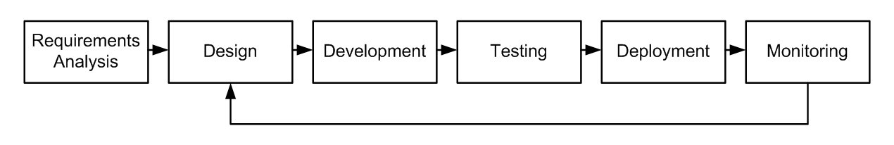
Designing and implementing logistics operations, complex processes, and systems involves several steps.
There is often a feedback loop involved, which allows to refine/improve/extend the system.

Requirements Analysis

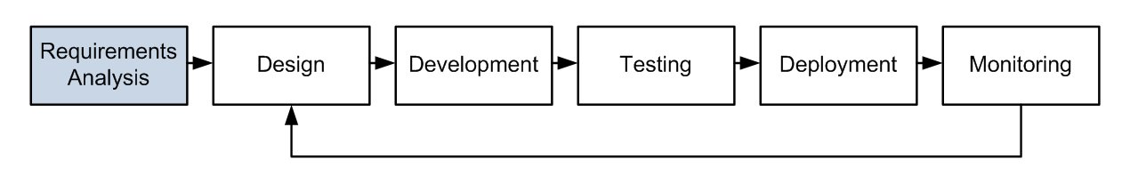
Understand the problem domain and specifications, and identify the key entities involved.
Build an abstract representation of the system to be able to handle various input scenarios.

System Design

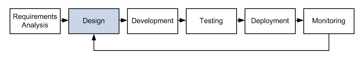
Divide the system into components; choose suitable methodologies for implementing each component.
Define appropriate data structures, input/output formats, and so on.

Development

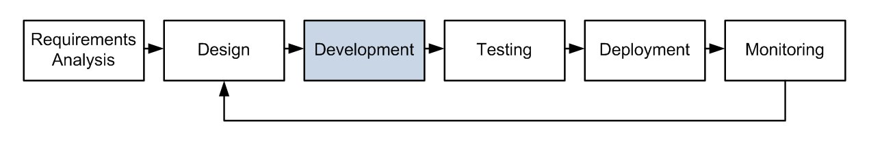
This is the actual implementation work and is typically coupled with some preliminary testing.
For source code, janitorial work, refactoring and some optimisations are also performed at this stage.

Testing

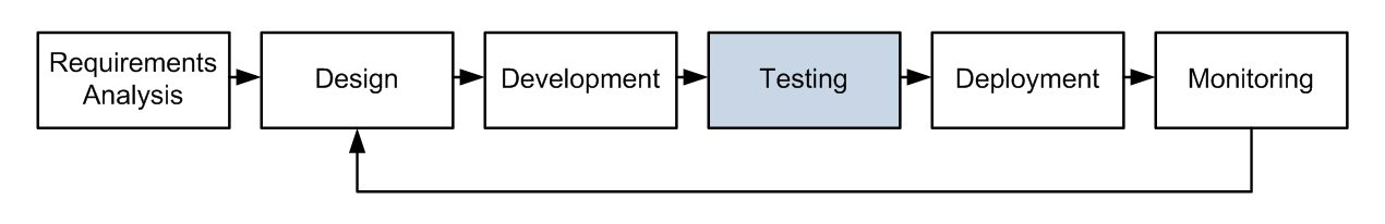
Validation is performed once the system is partially/ entirely developed; also benchmarking and profiling.
A system's performance evaluation is undertaken (experimentation with different inputs, distributions).

Deployment

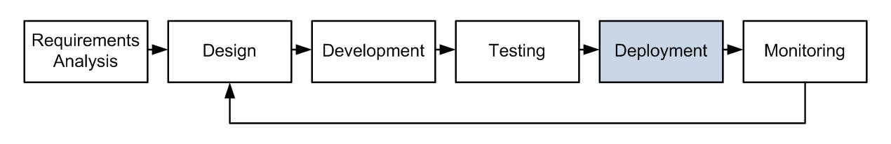
Once the tool (planner, simulator, etc.) has been thoroughly tested it can be deployed in a real setting.
The input will be based on actual data and inputs may change over time (e.g. based on certain events).

Monitoring

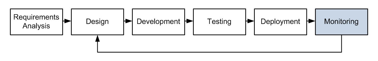
Once the system is operational, it is possible to gather real measurements and use those to refine the design.
If new requirements are identified during operation, the system can be further extended.

The Bin Service Process

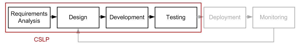
Your simulator will be implementing a good bit of what could become a real logistics system.
Unfortunately you will not have the opportunity to experiment with real data, but (time permitting) you have the flexibility to develop additional features.

Performance Evaluation

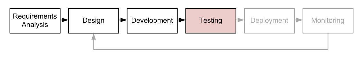
We have discussed the requirements, as well as different design and development aspects for your simulator.
We will now look into performance evaluation issues. Some of the things I will present may not be needed for this assignment, but will likely prove useful later.

Performance Evaluation

Generally speaking, this is about quantifying the performance of a system.
The first step is to identify the relevant metrics, i.e. measurable quantities that capture properties of interest.

This could the throughput of a network link, the power consumption of a mobile device, the memory used by a software application, etc.
For CSLP we are interested in the average trip duration, number of trips per schedule, trip efficiency, average volume collected, percentage of overflowed bins.

Metrics

It is essential to understand the performance evaluation goals, i.e. whether a metric should be small or large.
It is also important to be aware of the goals of the evaluation:

Improve the dimensioning/parametrisation of a system or process.
Compare how different designs perform under different inputs and chose the best one.

Methodologies

When designing a system, performance evaluation can be conducted through one or more of the following methodologies:

Numerical analysis - plugging some numerical values into a mathematical model of the system and computing the metrics of interest.
Simulation - constructing a simplified model of a more complex real system and simulating its behaviour; typically fast, but neglecting certain practical aspects.
Experimentation - Analysing the performance of a system via measurements. Assessing performance under exceptional circumstances may be infeasible.

Accuracy

It is advisable that the assumptions made for the evaluation campaign are well documented, to ensure the tests performed are reproducible.
You are working with a stochastic simulator and thus there will be some variability in the results of different tests with the same input.
For this practical you have been asked to give average values of a set of metrics.
In rigorous studies, it is necessary to also provide some confidence intervals for the results.

Summary Statistics

Histograms are graphical representations of the distribution of a set of measurements.

Example: distribution of the h-index of Nobel-prize recipients in Physics between 1985-2005.

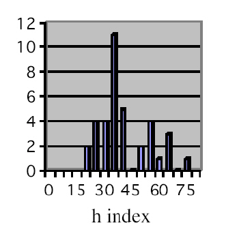
Source: J.E. Hirsch, "An index to quantify an individual's scientific research output", Proc. NAS, 2005.

h-index: number of papers with h or more citations.

Histograms

In mathematical terms, the histogram is a function that counts the number of observations in different categories (bins – not to be confused with waste bins in simulator)
The number of bins is typically computed as

$$k = \frac{\max(\mathbf{x}) - \min(\mathbf{x})}{\sqrt{n}}$$

where n is the number of samples in the data set $x$.

Mean and Standard Deviation

Computing the mean (average) of a set of measurements is straightforward:

$$\mu = \frac{1}{n}\sum_{i=1}^n x_i $$

The standard deviation gives a measure of the variation of the measurements from the mean:

$$ \sigma = \sqrt{\frac{1}{n}\sum_{i=1}^n (x_i - \mu)^2}$$

Confidence Intervals

These can be used to quantify the uncertainty about the average of a set of measurements subject to randomness.
When computing averages across multiple simulations, you are gathering samples to estimate an unknown population mean.
You choose the significance level that will reflect how confident you can be that the true value lies within that interval,
E.g. for a significance level of 0.05, you will obtain a 95% confidence interval (typically used in practice).

Confidence Intervals

The width of the confidence is affected by:

sample size,
population variability (standard deviation),
confidence level chosen.

Central Limit Theorem: For a large sample size, the sampling distribution of the mean will approach a normal distribution.
The sample mean and the mean of the population are identical.

Confidence Intervals

A quick method to compute a CI is:

$$\mu \pm z_{\alpha/2}\frac{\sigma}{\sqrt{n}}$$

where $z_{\alpha/2}$ is the critical coefficient corresponding to a confidence level $\alpha$; and is obtained from z-score tables.

Example: Sample size 20, mean 10, standard deviation 1.45, 95% confidence level, i.e. a critical coefficient corresponding to a z-score of 0.475, which is 1.96.

CI is 20±0.02

i.e. [19.8, 20.2]

Confidence Intervals

Plotting CIs

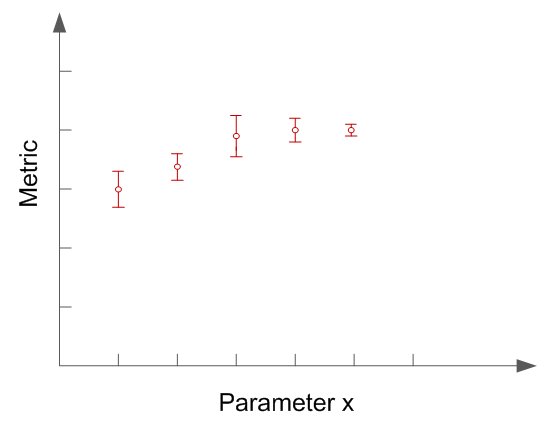
Notes on Unit Testing

Unit Testing

This refers to testing different components (units) you develop;
More common in large collaborative projects where different people are responsible for different (independent) functionality;
Goal: verify that a particular component works as expected:

The output returned makes sense / is correct;
Errors are handled appropriately.

Typically involves writing a tests suite, which one can run at any stage.

Unit Testing

If you later decide to add more functionality, well tested code will allow you to easily identify limitations of the new features.
You will probably develop separate new tests for the new features.
The only cost is time: you need time to write these tests, but the quality of the resulting software may be worth it.

What's involved

Many languages offer unit testing frameworks
– see list here.
Sometimes use stubs / mock objects to isolate a particular unit of work you want to test.
The idea is to implement some abstract interface that simply allows the component you are testing to work, without actually doing anything.
Similarly you may also implement drivers, which primarily call the unit you want to test.

A Java example

Suppose you want to test this:


public class Summator{
  public int computeSum(int[] values) {
    int sum = 0;
    for (int item : values)
      sum += item;
    return sum;
  }
}

A Java example

Prepare the test


import static org.junit.Assert.assertEquals;
import org.junit.Test;

public class TestOne {
  @Test
  public void checkResult() {
    Summator s = new Sumator();
    int[] numbers = {1,2,3,5,7};
    int result = s.computeSum(numbers);
    assertEquals(18, result);
  }
}

A Java example

Running the test outputs


iJUnit version 4.12
.
Time: 0,006

OK (1 test)

A Java example

Assuming you modify the code of the 'Summator' (e.g. return before computing anything) and then re-run the test:


JUnit version 4.12
.E
Time: 0,007
There was 1 failure:
1) checkResult(TestOne)
java.lang.AssertionError: expected:<18> but was:<0>
  at org.junit.Assert.fail(Assert.java:88)
  ...

FAILURES!!!
Tests run: 1,  Failures: 1

This tells you the number of failures, where the problems were, and what went wrong.

Final remarks

Admittedly you may not need sophisticated unit testing for CSLP, but if you want to learn more, the JUnit wiki is a good place to start.
PyUnit gives you the Python version of JUnit. Similar frameworks available for other languages.
You may even want to take a test driven development (TDD) approach, i.e. write a test; see the code fail; write code to pass the test; repeat.

Results Visualisation

At the beginning of this course, the large majority of respondents to the survey had no experience with visualisation/plotting tools, or found this challenging.
Wide range of software suitable for such purposes.
As always, ease of use is traded for the number of features supported and quality of end results.
For CSLP you may use things as simple as charts generated with spreadsheet tools (LibreOffice Calc, Microsoft Excel, OS X Numbers, Google Sheets, etc.),
or work with specialised software/packages/statistical computing languages (gnuplot, Matlab, matplotlib, R).

Results Visualisation

Like with other things, the visualisation tool is mostly a personal choice.
Though at times you may be required to use a specific tool (employer/project request or license constraints).
If you work collaboratively, open-source, cross-platform portable solutions are certainly appropriate.

Plotting with R

Today I will give a short guide to R, since

It meets the aforementioned criteria;
You will likely use this tool for other projects where you will need to process and visualise data sets.

R is increasingly popular among data analysts and statisticians.
Workflow can be simplified with the use of graphical front-ends such as RStudio (as you type help, partial script execution, exporting images, etc.).
As you become more expert, you can combine it with C/Java/Python code.

Plotting with R

Once you installed R (already installed on DiCE), you can invoke different functions through a CLI.


$ R
...
Type 'demo()' for some demos, 'help()' for on-line help, or
'help.start()' for an HTML browser interface to help.
Type 'q()' to quit R.

>

Though perhaps more often you will write some scripts.
Even if using a graphical front-end, you still have the console, which is handy if you need to install packages.

R packages

DiCE machines should have most packages you would require, but for your personal installation, you may have to install some manually.
For instance, you may want to install the ggplot2 package to produce complex graphics more easily.
The procedure is pretty straightforward:


> install.packages("ggplot2")

This takes care of all the necessary download, compilation, and installation for you.

Writing a simple (yet useful)
R script

Writing a simple script

Say we have some delays you recorded in a file named 'values.dat' and you want to see if they follow a certain distribution.
Imagine a file like this


delay
78
500
13
190
95
 ...

Where first line contains the name of variable observed.
We expect the delays stored in this file to follow an Erlang distribution with shape $k=2$ and rate $\lambda=1/100$.

Writing a simple script

First thing we do is to read these values from the file


measurements <- read.delim("values.dat")

Then obtain an estimate of the Probability Density Function (PDF) for the values corresponding to the 'delay' object in the dataset.


empiricalDistr <- density(measurements$delay)

The 'density' function is implementing a kernel density estimator (though no need to worry about the details).

Writing a simple script

Next we obtain an 'ideal' PDF of an Erlang-2 random variable with rate $\lambda=1/100$, where say we are interested in delays ranging between 0 and 500 seconds.


span <- seq.int(0, 500, length.out=500)
idealDistr <- dgamma(span, 2, rate=1/100)

Here we are actually drawing from a gamma distribution, but since the shape is an integer ($k=2$) gamma and Erlang are equivalent.

Writing a simple script

What remains is only to plot the two curves
```
plot(span, idealDistr, type="l", 
  col="red", lwd=2, 
  xlab="Delay [s]", ylab="Probability", main="PDFs")
lines(empiricalDistr, col="blue", lwd=2)
```
where we plot with lines (of width 2), use red for the 'ideal' PDF and blue for the empirical distribution, and label the axes accordingly.
Finally set the legend


legend(370, 0.0035, legend=c("Ideal", "Empirical"),
       col=c("red", "blue"), lty=1:1, lwd=2:2, cex=1.2)

Writing a simple script

Putting everything together, the following script...


measurements <- read.delim("values.dat")

empiricalDistr <- density(measurements$delay)

span <- seq.int(0, 500, length.out=500)

idealDistr <- dgamma(span, 2, rate=1/100)

plot(span, idealDistr, type="l", col="red", lwd=2, 
  xlab="Delay [s]", ylab="Probability", main="PDFs")
lines(empiricalDistr, col="blue", lwd=2)

legend(370, 0.0035, legend=c("Ideal", "Empirical"),
       col=c("red", "blue"), lty=1:1, lwd=2:2, cex=1.2)

Writing a simple script

...produces this figure

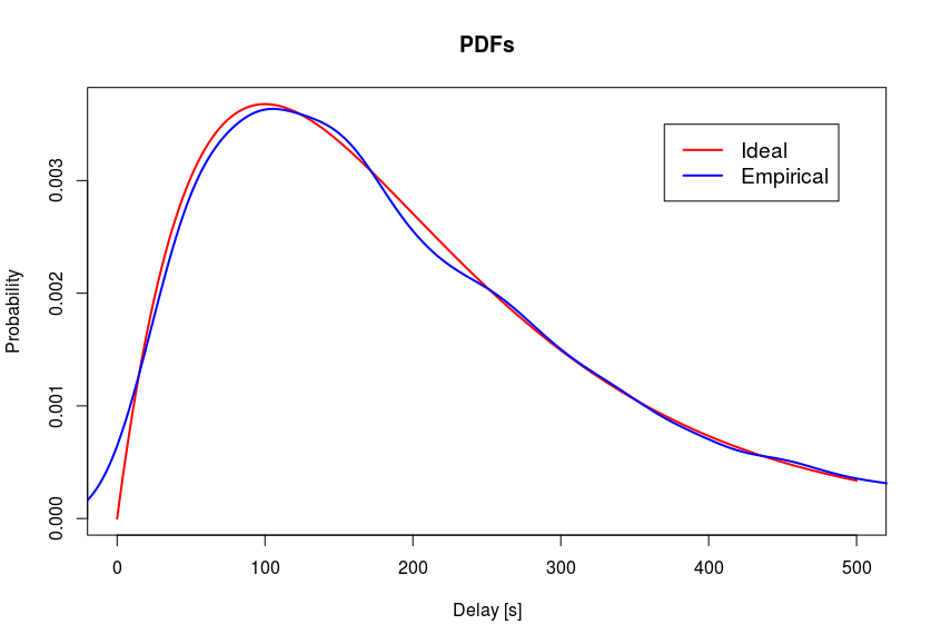
Producing fancier plots

Say you want to plot the time evolution of some metric at two different agents.
E.g. the throughput of two stations in a Wi-Fi network, when one of them changes the PHY rate.
Data stored in a CSV file, first column time (in seconds), 2nd and 3rd column stations' throughputs (in kb/s).
The file would look like the following:


  
 10.000, 1.208e+04, 1.205e+04
 11.000, 1.196e+04, 1.207e+04
 12.000, 1.221e+04, 1.196e+04
 13.000, 1.189e+04, 1.230e+04
 14.000, 1.188e+04, 1.226e+04
 15.000, 1.189e+04, 1.261e+04
 ...

Producing fancier plots

First load the libraries needed.


library(ggplot2)
library(reshape2)

Prepare file path and read the contents of the file.


folder = "results" # location of data files

# read from CSV file
# filename obtained through concatenation
contents <- read.csv(paste0(folder, "/throughput.dat"), 
		header=F)

Set suggestive names for the objects.


names(contents) <- c("time", "STA 1", "STA 2")

Producing fancier plots

Create an empty data frame and combine with read data.


# create empty data frame
mydata <- data.frame()

# combine objects
mydata <- rbind(mydata, contents)

Time logged started at 10s, so make adjustment to display more elegantly.


# adjust time to display
mydata$time <- mydata$time - 10

Producing fancier plots

Produce the plot...


myplot <- ggplot(melt(mydata, id="time"), 
  aes(x=time, y=value/1e3)) + 
  geom_line(aes(colour=variable)) + 
  scale_x_continuous(limits=c(0,250)) +
  scale_y_continuous(limits=c(0,15)) +
  ylab("Throughput [Mb/s]") +
  xlab("Time [s]") +
  theme_bw() +
  theme(plot.margin = unit(c(0.5,1,0,0.5), "lines"),
        plot.background = element_blank(), 
	legend.title=element_blank(),
        legend.position="top", 
        text = element_text(size=20)) + 
  scale_color_manual(values=c("cadetblue4", "coral4"))

... OK, a lot to take in here! Let's go through this step by step.

Using the `ggplot` function

First we need to convert data object into a molten data frame, telling the plotter the variable changing is 'time'.


myplot <- ggplot(melt(mydata, id="time"), 
...

Then construct aesthetics mapping, i.e. x and y axes. We want to plot in Mb/s, so we need to divide throughput values by 1,000.


  aes(x=time, y=value/1e3)) + 
...

Instruct to connect the variables in order specified by x axis, with lines; allow different colours for each.


  geom_line(aes(colour=variable)) + 
...

Using the `ggplot` function

Set ranges for the x and y axes, and label these.


  scale_x_continuous(limits=c(0,250)) +
  scale_y_continuous(limits=c(0,15)) +
  ylab("Throughput [Mb/s]") +
  xlab("Time [s]") +

Set a simple theme, adjust the margins slightly, no background


  theme_bw() +
  theme(plot.margin = unit(c(0.5,1,0,0.5), "lines"),
        plot.background = element_blank(), 
...

Using the `ggplot` function

No legend title, place the legend at the top, increase font size to improve readability


	legend.title=element_blank(),
        legend.position="top", 
        text = element_text(size=20)) + 
...

Finally, set some custom colours


  scale_color_manual(values=c("cadetblue4", "coral4"))

And now plot the chart.


  plot(myplot)

End result

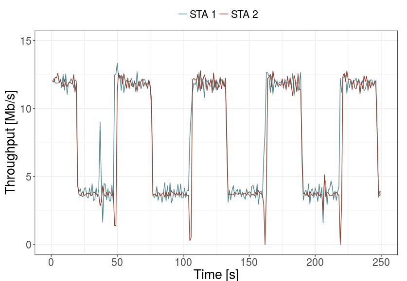
Bar plots & error bars

Now let's try something more complex.
Say we want to compare the latency performance of two network protocols, when a client downloads files of different sizes.
With each protocol, we download every file and measure the delay over 10 such experiments.
We are interested in the average and standard deviation of the latency measured.

Bar plots & error bars

Files containing these measurements for each protocol will look like this


256kB	00.23
256kB	00.19
...
512kB	00.52
512kB	00.42
...
...
4096kB	03.30
4096kB	04.29

Bar plots & error bars

As before, we first extract and label the data


mydata_1 <- read.delim(paste0(folder, 
		"/latency_1.dat"), header=F)
mydata_2 <- read.delim(paste0(folder, 
		"/latency_2.dat"), header=F)

names(mydata_1) <- c("FILESIZE", "LATENCY")
names(mydata_2) <- c("FILESIZE", "LATENCY")
mydata_1$what = "Protocol 1"
mydata_2$what = "Protocol 2"

Then prepare empty data frames to store the average and standard deviation values of the measured latency


avg_lat <- data.frame()
std_lat <- data.frame()

Bar plots & error bars

Next, subset the data using the different file sizes


for(file in unique(mydata_1$FILESIZE)) {
  tmp_1 <- subset(mydata_1, FILESIZE==file)
  tmp_2 <- subset(mydata_2, FILESIZE==file)

Compute the means for each protocol and bind data


  avg_lat = rbind(avg_lat, rbind(c(what="Protocol 1", 
		    FILESIZE=file, 
                    LATENCY=mean(tmp_2$LATENCY)), 
                c(what="Protocol 2", FILESIZE=file,
                    LATENCY=mean(tmp_1$LATENCY))))

and do the same for standard deviations


  std_lat = rbind(std_lat, rbind(c(what="Protocol 1", 
		    FILESIZE=file, 
                    LATENCY=sd(tmp_2$LATENCY)), 
                c(what="Protocol 2", FILESIZE=file, 
                    LATENCY=sd(tmp_1$LATENCY))))  
}

Bar plots & error bars

Recall we need molden data frames for ggplot


dd_avg_lat <- melt(avg_lat, id=c("what", "FILESIZE"))
dd_std_lat <- melt(std_lat, id=c("what", "FILESIZE"))

The error bars should correspond to $\mu \pm \sigma$. Therefore we need to compute the boundaries of the error bars.


dd_avg_lat$ymax <- as.numeric(dd_avg_lat$value) + 
	as.numeric(dd_std_lat$value)
dd_avg_lat$ymin <- as.numeric(dd_avg_lat$value) - 
	as.numeric(dd_std_lat$value)

We should now have everything we need for plotting.

Bar plots & error bars

We want to plot the average latency with boxes (bar), as a function of the file size


myplot <- ggplot(dd_avg_lat, aes(x=as.character(FILESIZE), 
  y=as.numeric(value))) + 
  geom_bar(aes(fill=what), position = "dodge", stat="identity") + 
  geom_bar(aes(fill=what), position = "dodge", stat="identity", 
  colour="black") +

Here we use bar chart geometry; we want to avoid overlap (hence 'dodging' bars side by side),
Force the height of the bars to the value of the data ('identity').
First bars will have a coloured fill, second bars black contours around these.

Bar plots & error bars

We add the error bars next, centring on the boxes, adjusting width of the ends and line.


  geom_errorbar(aes(ymax=ymax, ymin=ymin, fill=what ),  
	position=position_dodge(.9), width=0.25, lwd=1) +

Custom tics on the x axis


scale_x_discrete(limits=c("256kB", "512kB", "1024kB", 
	"2048kB", "4096kB")) +

Labelling the axes


  ylab("Download time [s]") + xlab("File size") +

Bar plots & error bars

Finally setting the theme, legend position, font size, etc.


  theme_classic() +
  theme(legend.title=element_blank(), 
	legend.position=c(0.15,0.9), 
	legend.background = element_rect(), 
        text = element_text(size=20)) +

and custom colours.


  scale_fill_manual(values=c("cadetblue", "coral")))

Bar plots & error bars

The complete call


myplot <- ggplot(dd_avg_lat, aes(x=as.character(FILESIZE), 
  y=as.numeric(value))) + 
  geom_bar(aes(fill=what), position = "dodge", stat="identity") + 
  geom_bar(aes(fill=what), position = "dodge", stat="identity", 
    colour="black") + 
  geom_errorbar(aes(ymax=ymax, ymin=ymin, fill=what ),  
    position=position_dodge(.9), width=0.25, lwd=1) +
  scale_x_discrete(limits=c("256kB", "512kB", "1024kB", 
    "2048kB", "4096kB")) +  
  ylab("Download time [s]") + xlab("File size") + 
  theme_classic() +
  theme(legend.title=element_blank(), legend.position=c(0.15,0.9), 
     legend.background = element_rect(), 
     text = element_text(size=20)) +
  scale_fill_manual(values=c("cadetblue", "coral"))

...et voila!

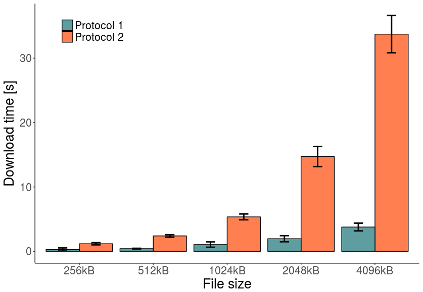
Additional resources & remark

If you feel R is for you and want to learn how to produce even more sophisticated charts, lots of tutorials and examples are available on the R-bloggers web site.
Everything you need to know about ggplot2 features is explained here.
NB: You are not required to produce plots of the results you obtain for CSLP using R. You can use any tool you like, though R may prove useful for future projects as well.

Part 3 requirements

Part 3 submissison

Part 3 carries 50% of the total marks
Deadline: Wed 21 st December, 2016 at 16:00
(unless ITO/year organiser gave you an extension)
Wise to check again and comply with the University academic misconduct policy.
Remember this is an individual project.
Reusing publicly available code is OK, but clearly mark the parts you did not author yourself.

Part 3 requirements

By the part 3 deadline you are expected to have:

A complete and working version of the simulator.
A short written report (in PDF format) documenting your implementation and key findings.

Your code will not be tested for functionality you were expected to have at Part 2, but will be expected to work on valid input files provided as command line arguments.

Functionality expected for Part 3

Correct lorry scheduling, bin service, and route planning;
Correct summary statistics, in line with output format specification;
Experimentation support;
Test files non-trivially different from each;
Evidence of reasonable run times and optimisation;
Appropriate indentation and spacing, no dead code;
Evidence of appropriate use of source control.

Written report

Do not write an overly lenghty report;
Avoid putting code; If you really need to explain something non-trivial, use an appendix;
Briefly document the architecture of your simulator (you may already have this by now), your design choices, and testing efforts;
Briefly discuss experiments performed, results obtained (potentially accompanied by plots), and insights gained;
Document any additional features you implemented (extra credit for these).