CNV: Dichromatic Vision project option for assignment 2

This page describes one of the possible project options for assignment 2; please read the general project description first before looking at this specific project option.

Background

Humans and macaque monkeys have trichromatic color vision, with three different cone types in daylight vision, each responding best to different wavelengths of light. The three cone types are typically labeled L, M, and S (long, medium, or short-wavelength), or (very loosely) RGB (red, green, or blue). Most other mamals, including New World monkeys, have only two, namely S and and another type that can be called ML, similar to color-blind humans.

Most studies of color vision use the macaque, due to its similarity to humans, but it is interesting to consider the similarities and differences with vision in other mammals, as well as with colorblind humans. At least two imaging studies have looked at dichromatic color vision, Johnson et al (2010), who studied the tree shrew, and Buzas et al. (2008), who studied the marmoset. These studies show various similarities and differences between the dichromatic and trichromatic species.

There have been models of the self-organization of color preferences in V1 of macaque, such as De Paula (2007), but I have not yet seen any model of color preferences in a dichromatic animal. The purpose of this project is very open ended, but basically involves adapting an existing trichromatic model to use two cone classes, and analyzing the result. Part of the assignment is to try to come up with a suitable scientific question to pose that could be answered by such a model, which could focus on the spatial organization, the response to different stimuli, or some other aspect of the model.

GCAL LMS color simulation

To get you started, I've provided a model definition script gcal_or_cr.ty for a simple trichromatic simulation based on the subcortical color pathways modeled by De Paula (2007), with that study's LISSOM V1 replaced with the GCAL V1 from Stevens et al. (2013). You can use this file with any recent version of Topographica, such as the copy installed in /group/teaching/cnv/topographica. To try it out using the Tk GUI, follow these steps:

First, the simulation uses images stored in /group/project/csng/images/mcgill on DICE; you'll need to make that directory show up in your images folder (~/topographica/images/ if you followed the DICE instructions for assignment 1) by running:
```
  cd ~/topographica
  ln -s /group/teaching/cnv/topographica/images/mcgill ./images/
```
If you are using a non-DICE machine, you'll need to copy the images to the corresponding location in your installation. These files contain the estimated Long, Medium, and Short-cone activations of humans in response to photographs of natural scenes, from the McGill Calibrated Color Image Database.
Save a copy of the gcal_or_cr.ty example file into your topographica directory (~/topographica/gcal_or_cr.ty on DICE), and launch it:
```
  cd ~/topographica
  ./topographica -g gcal_or_cr.ty
```
To see the network, you can look at it in the Model Editor, though the text labels are long and hard to read without moving the sheets around:

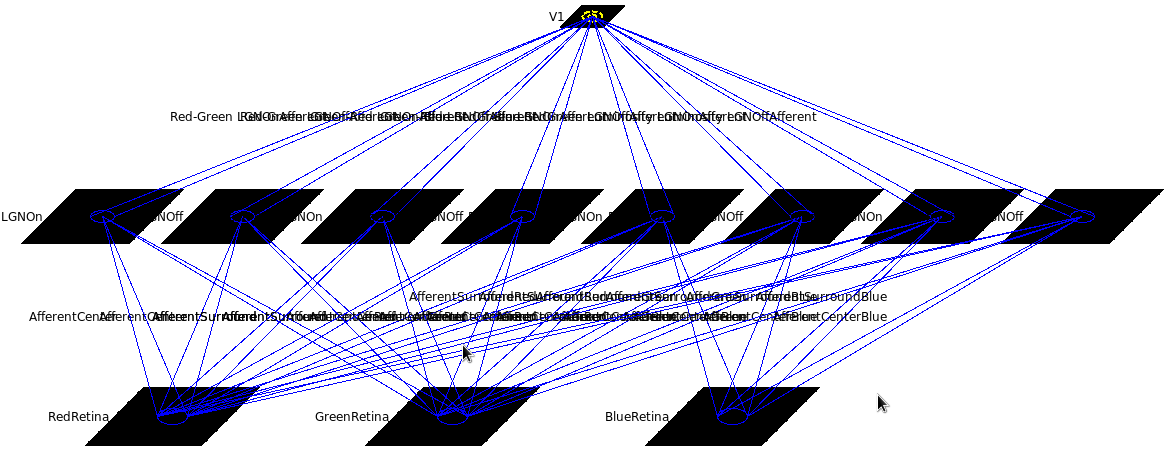
This model has three cone photoreceptor types, and eight LGN channels: 6 color opponent, namely Red On center/Green Off surround (labeled "Red-Green LGNOn"), Green On center/Red Off surround (labeled "Green-Red LGNOn"), Blue On center/(Red+Green Off surround) (labeled "Blue-RedGreen LGNOn"), and the same with On and Off switched, plus 2 monochrome (labeled "Luminosity LGNOn" and "Luminosity LGNOff") channels. All of these channels have similar structure, differing only in the specific combination of center and surround Gaussian-shaped CFs they have from the cones. All of these LGN channels then project to V1.
You should the run the network for a few iterations in the GUI and look at the activity and eventually Projection plots to see what it does, how it compares to monochromatic GCAL from the first assignment, and generally make sure that it seems to be working ok and that you understand the structure.
You can run it for a few thousand iterations in the GUI until it self-organizes, and can then visualize a Hue map just as for orientation in the first assignment, either by selecting the "Hue Preference" map in the GUI, or by running "measure_hue_map()" from the command line. Once the hue map has been measured, the orientation map can be plotted without further measurement, because measure_hue_map also varies orientation. Here are the results from iteration 5000, using the default "-p color_strength=0.75 -p 'cone_scale=[0.90,1.00,0.97]'" (described below):

Hue preference Hue preference and selectivity Orientation preference Orientation preference and selectivity

For comparison, here are the resuls from "-p color_strength=0.4 -p 'cone_scale=[0.93,1.03,1.04]'", which weights the color-opponent channels less and balances the three cone types to try to get a rainbow of hues in each blob:

Hue preference Hue preference and selectivity Orientation preference Orientation preference and selectivity
You can keep going in the GUI, but it's usually easier to run gcal_or_cr.ty in batch mode instead (or you can start setting up an IPython notebook for this if you like, or use Lancet). Sample batch mode command for running to simulation time 5,000 (which is usually sufficient to see how it will organize) and analysing the map at times 1,000 and 5,000:
```
  cd ~/topographica
  ./topographica -a -c "run_batch('gcal_or_cr.ty',color_strength=0.75,cone_scale=[0.90,1.00,0.97],times=[1000,5000])"
  
```
This command takes 8 minutes on my Core i3 machine, but could be more if your machine is slower or heavily loaded. The color_strength and cone_scale arguments here can be ommitted, as they are the default values.
The output from the simulation will be in ~/Topographica/Output/201403052333_gcal_or_cr by default (note the capital T), where 201403052333 is the year, month, day, hour, and minute when the command was started (to provide a unique tag to keep track of results). The output directory name should be printed to your terminal, so you can just cut and paste from there. When it's done, be sure to examine the .out file in that directory, so that you can detect any warnings that might be important (such as parameters that you thought you changed but the code warns you were not actually changed due to typos). You can use your favourite image viewer to see the .png images, such as hue maps, orientation maps, and weight plots.
For instance, if you're using gthumb, you can do gthumb *.png. For gthumb, it works better if you go to the Preferences and set the Viewer options to have a Zoom quality of Low (to avoid smoothing) and After loading an image to Fit image to window (so that it's large enough to see). You'll at least want to look at the various Hue and Orientation plots from the latest iteration, but the rest are also useful.
If the images make it look like this might be a useful network, then you can then load the saved snapshot to further explore what it does:
```
  ./topographica -g -c "load_snapshot('$HOME/topographica/Output/201303011200_gcal_or_cr/201303011200_gcal_or_cr_05000.00.typ')"
  
```
Or you can build an IPython notebook to explore the simulation, based on those used in the first assignment, which is a good way to start collecting results.

Improving this simulation is the subject of a PhD thesis currently underway, which has turned out to be complex and to involve a lot of subtle issues about how color is processed at the various subcortical stages. So the model in this assignment has a number of important limitations, but it does successfully organize color and orientation preference maps, and so it should work for the proof of concept required for this assignment.

Important notes:

By default, this simulation uses a single eye, but it can be made binocular by setting eyes=['Left','Right'], in case you need to investigate a question requiring two eyes.
By default, this simulation does not use gain control, since parvo cells (the more color selective cells) are not normally thought to exhibit gain control. You can set gain_control=True if you wish.
The simulation is biased towards color by default, making the color map well organized at the expense of the orientation map, because there are six color-opponent LGN channels and two luminosity channels (which receive inputs from all cone types), each weighted equally by default. This balance can be changed by the color_strength parameter, as shown above, though you will need to balance the hue representation using cone_scale (below) if you do.
The balance across the hue spectrum at a given color_strength can be adjusted by changing the brightness scale of each cone type using the cone_scale parameter; the current values were chosen by De Paula. E.g. to get a stronger representation of blue hues, you can set cone_scale=[0.9,0.9,1.2]. Tuning the model in this way is arbitrary and thus not very satisfying, but the right way to achieve such a color balance requires homeostatic mechanisms that we are not yet done modelling, so it's the best we have for now.
The measurement of the hue map is overly simplistic, and is difficult to interpret as a physical process. To see what it does, open a Hue Preference window and an Activity window in the Tk GUI and then hit the Refresh arrow in the Hue Preference window. Basically, it goes through the various values of Hue in HSV space, activating the L, M, and S cone photoreceptors in the model (labeled "Red", "Green", and "Blue" with the RGB equivalent for each HSV value, measuring the responses in V1. This procedure amounts to activating each of the cone types as if there were no correlations between them, when in fact the L and M channels will both be activated by most hues in the real world. Thus it is difficult to interpret the results of this procedure as true physical hue preferences; instead it is really telling us which combinations of cone activations are preferred by the various neurons in V1. But it does at least demonstrate differences in V1 preferences, and is a starting point. We have developed much more realistic color map measurement techniques, but these are too complicated to use in this assignment. In any case, there are no experimental results showing a proper hue map directly anyway, so this map should be considered a useful way to understand how the model works, rather than a simulation of a physical process.

GCAL MS color simulation

The gcal_or_cr.ty LMS simulation can easily be converted to an MS simulation by overriding the parameter cone_types (['Red','Green','Blue'] by default) with cone_types=['Green','Blue'], as in:

./topographica -a -c "run_batch('gcal_or_cr.ty',cone_types=['Green','Blue'],times=[1000,5000])"

This change removes the Red (Long) input cone type, replaces the previously color-opponent Red-center/Green-surround and Green-center/Red-surround LGN channels with spatially opponent Green-center/Green-surround channels, and replaces the Blue/(Red+Green) channels with Blue/Green channels. The Luminosity channels ares now (Green+Blue center)/(Green+Blue surround).

If you run this model and look at the Hue preference map, you can see that just about the only Hue preference found is now blue, which makes sense given the only color-opponent LGN cell type remaining, the Blue-center/Green-surround cells. But one might also expect to have cells selective for "not blue", i.e. yellow or green, since there are both ON and OFF versions of the Blue-center/Green-surround cells. Adjusting the cone channel strengths may restore some of the green responses, but this has not been tested.

You can now take this simulation and do whatever you like with it, either based on biological data or on a theoretical idea. The first thing to do is to consider whether this set of LGN channels is what you really want to use. E.g. do you really want to have Luminosity channels? The evidence for a channel connecting equally to all cone types is not clear, and it's worth considering eliminating it. The luminosity channel can be disabled using color_strength=1.0, or eliminated altogether in the file. Similarly, are the Green/Green and Blue/Green channels the right ones to have for the species you're modelling? You'll have to do some literature searching to find out. If not, change them! The given file is just a starting point, and has not been compared with or validated against any particular dichromatic species.

Modelling project

Once you have a dichromatic simulation, the scientific question to be addressed in this assignment is completely open. For instance, is there anything that you can see from the experimental studies that can easily be investigated computationally? If so, do so. E.g. perhaps the anatomical evidence for certain pathways is unclear, in which case you can try them both out and try to understand how the two alternatives change the results.

Or, are there clear differences between dichromat and trichromat species, in V1 map organization or V1 preference types? If so, see if your proposed dichromatic architecture exhibits the observed differences, compared to the original trichromatic simulation.

Any similar question can be investigated, and you can then report the results. Whether the results were as expected or not, you should think about your network, observe the patterns of activity and connectivity, and decide if you believe it is an appropriate model for what you're looking at. Basically, you're trying to (a) build a decent model that includes the mechanisms that at least might result in the phenomenon you're investigating, (b) determine whether it does so, and (c) analyse what those results depend on -- why they occur.

Whatever you end up investigating, in your report, you'll need to make it clear what question(s) you were addressing, demonstrate that the model was a reasonable first approach to investigating those questions, explain how the model's mechanisms relate to processes in animal V1, and explain why the results you observe (whether they match previous data or not) occur. Once you're ready, you can report and submit your results as outlined in the general project description.


Hue preference	Hue preference and selectivity	Orientation preference	Orientation preference and selectivity