MLPR → Course Notes → w8d
PDF of this page
Previous: Bayesian logistic regression and Laplace approximations
Next: Variational objectives and KL Divergence
$$\notag
\newcommand{\D}{\mathcal{D}}
\newcommand{\E}{\mathbb{E}}
\newcommand{\M}{\mathcal{M}}
\newcommand{\N}{\mathcal{N}}
\newcommand{\be}{\mathbf{e}}
\newcommand{\bm}{\mathbf{m}}
\newcommand{\bw}{\mathbf{w}}
\newcommand{\bx}{\mathbf{x}}
\newcommand{\g}{\,|\,}
\newcommand{\intd}{\;\mathrm{d}}
\newcommand{\sth}{^{(s)}}
\newcommand{\te}{\!=\!}
$$
Computing logistic regression predictions
In the previous note we approximated the logistic regression posterior with a Gaussian distribution. By comparing to the joint probability, we immediately obtained an approximation for the marginal likelihood \(P(\D)\) or \(P(\D\g\M)\), which can be used to choose between alternative model settings \(\M\).
Now we return to the question of how to make Bayesian predictions (all implicitly conditioned on a set of model choices \(\M\)): \[\begin{align}
P(y\g \bx, \D) &= \int p(y,\bw\g \bx, \D)\intd\bw\\
&= \int P(y\g \bx,\bw)\,p(\bw\g\D)\intd\bw.
\end{align}\]
We can approximate the posterior with a Gaussian, \(p(\bw\g\D)\approx \N(\bw;\,\bm, V)\), using the Laplace approximation (previous note) or variational methods (next note). Using this approximation, we still have an integral with no closed form solution: \[\begin{align}
P(y\te1\g \bx, \D) &\approx \int \sigma(\bw^\top\bx)\,\N(\bw;\,\bm, V)\intd\bw\\
&= \E_{\N(\bw;\,\bm, V)}\!\left[ \sigma(\bw^\top\bx)\right].
\end{align}\] However, this expectation can be simplified. Only the inner product \(a\te\bw^\top\bx\) matters, so we can take the average over this scalar quantity instead. The linear combination \(a\) is a linear combination of Gaussian beliefs, so our beliefs about it are also Gaussian. By now you should be able to show that \[
p(a) = \N(a;\; \bm^\top\bx,\; \bx^\top V\bx).
\] Therefore, the predictions given the approximate posterior, are given by a one-dimensional integral: \[\begin{align}
P(y\te1\g \bx, \D) &\approx \E_{\N(a;\;\bm^\top\bx,\; \bx^\top V\bx)}\left[ \sigma(a)\right]\\
&= \int \sigma(a)\,\N(a;\;\bm^\top\bx,\; \bx^\top V\bx)\intd{a}.
\end{align}\] One-dimensional integrals can be computed numerically to high precision.
Murphy Section 8.4.4.2 reviews a further approximation (derivation non-examinable), which is quicker to evaluate and provides an interpretable closed-form expression: \[
P(y\te1\g \bx, \D) \approx \sigma(\kappa\, \bm^\top\bx), \qquad \kappa = \frac{1}{\sqrt{1+\frac{\pi}{8}\bx^\top V\bx}}.
\] Under this approximation, the predictions use the mean weights \(\bm\) from the Gaussian approximation. If we used the Laplace approximation, we’re using the most probable or MAP weights. However, the activation is scaled down (with \(\kappa\)) when the activation is uncertain, so that predictions will be less confident far from the data (as they should be).
A route to avoiding Gaussian approximations is to approximate the prediction, which is an expectation, with an empirical average over samples: \[\begin{align}
P(y\g \bx, \D) &= \int P(y\g \bx,\bw)\,p(\bw\g\D)\intd\bw\\
&= \E_{p(\bw\g\D)}[P(y\g \bx,\bw)]\\
&\approx \frac{1}{S}\sum_{s=1}^S P(y\g \bx,\bw\sth), \quad \bw\sth\sim p(\bw\g\D).
\end{align}\] Our prediction is the average of the predictions made by \(S\) different plausible model fits, sampled from the posterior distribution over parameters.
However, it is not at all obvious how to draw samples from the posterior over weights for general models. For simple versions of linear regression, we know that \(p(\bw\g\D)\) is Gaussian, but we don’t need to approximate the integral in that case. For logistic regression there’s no obvious way to draw samples from the posterior distribution (if we don’t approximate it with a Gaussian).
A family of methods, widely used in Statistics, known as Markov chain Monte Carlo (MCMC) methods, can be used to draw samples from the posterior distribution for models like logistic regression and neural networks. MCMC was once part of the MLPR course, but won’t be on the exam this year. If you’re interested, I have tutorials online: https://homepages.inf.ed.ac.uk/imurray2/teaching/15nips/ — or an older version, but with a better recording: http://videolectures.net/mlss09uk_murray_mcmc/
Importance sampling is a simple trick you should understand, because it comes up in various contexts in machine learning beyond Bayesian prediction. Here we rewrite the integral as an expectation under an arbitrary tractable distribution of our choice, \(q(\bw)\): \[\begin{align}
P(y\g \bx, \D) &= \int P(y\g \bx,\bw)\,p(\bw\g\D)\,\frac{q(\bw)}{q(\bw)}\intd\bw\\
&= \E_{q(\bw)}\left[P(y\g \bx,\bw)\,\frac{p(\bw\g\D)}{q(\bw)}\right]\\
&\approx \frac{1}{S} \sum_{s=1}^S P(y\g \bx,\bw\sth)\,\frac{p(\bw\sth\g\D)}{q(\bw\sth)}, \quad \bw\sth\sim q(\bw).
\end{align}\] Here \(r\sth = \frac{p(\bw\sth\g\D)}{q(\bw\sth)}\) is the importance weight, which upweights the predictions for parameters that are more probable under the posterior than the distribution we sampled from.
We shouldn’t divide by zero, so we need \(q(\bw)>0\) when \(p(\bw\g\D)>0\). Moreover, we don’t want \(q(\bw)\ll p(\bw\g\D)\) for any region of the weights, or occasionally we would see an enormous importance weight, and the estimator will have high variance.
The final detail is that we can’t usually evaluate the posterior \[
p(\bw\g\D) = \frac{p(\D\g\bw)\,p(\bw)}{p(\D)},
\] because we can’t usually evaluate the denominator \(p(\D)\). However, we can approximate that using importance sampling! \[\begin{align}
p(\D) &= \int p(\D\g\bw)\,p(\bw)\intd\bw\\
&= \int p(\D\g\bw)\,p(\bw)\,\frac{q(\bw)}{q(\bw)}\intd\bw\\
&= \E_{q(\bw)}\left[\frac{p(\D\g\bw)\,p(\bw)}{q(\bw)}\right]\\
&\approx \frac{1}{S} \sum_{s=1}^S \frac{p(\D\g\bw\sth)\,p(\bw\sth)}{q(\bw\sth)} = \frac{1}{S} \sum_{s=1}^S \tilde{r}\sth,
\end{align}\] where we’ve introduced “unnormalized importance weights”, defined as: \[
\tilde{r}\sth = \frac{p(\D\g\bw\sth)\,p(\bw\sth)}{q(\bw\sth)}.
\] Substituting in this approximation to the Bayesian prediction, we obtain: \[
P(y\g \bx, \D) \approx \frac{1}{S} \sum_{s=1}^S P(y\g \bx,\bw\sth)\,\frac{\tilde{r}\sth}{\frac{1}{S}\sum_{s'=1}^S \tilde{r}^{(s')}}, \quad \bw\sth\sim q(\bw)
\] or \[
P(y\g \bx, \D) \approx \sum_{s=1}^S P(y\g \bx,\bw\sth)\,r\sth, \quad \bw\sth\sim q(\bw).
\] In this final form, the average is under the distribution defined by the ‘normalized importance weights’: \[
r\sth = \frac{\tilde{r}\sth}{\sum_{s'=1}^S \tilde{r}^{(s')}}.
\]
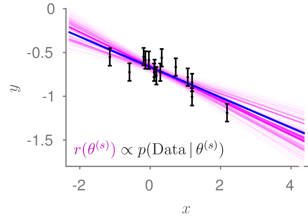
A special case might help understand importance sampling. If we sampled model parameters from the prior, \(q(\bw) = p(\bw)\), the unnormalized weights are equal to the likelihood, \(\tilde{r}(\bw) = p(\D\g\bw\sth)\).
We would sample some number, \(S\), settings of the parameters from the prior. Then we form a discrete distribution over these parameters with importance weights proportional to the likelihood. Functions that match the data will be given large importance weight.
Below is a linear regression example, where the true (unknown) line is shown in blue, and the purple lines show the discrete distribution over possible models we will use for prediction. The intensity of the lines indicate the importance weights. I drew 10,0000 samples from the prior, but most of the functions didn’t go near the data and were given such small weight that they are nearly white.
This importance sampling procedure works in principle for any model where we can sample possible models from the prior and evaluate the likelihood, including logistic regression. However, if we have many parameters, it is unlikely that any of our \(S\) samples from the prior will match the data well, and our estimates will be poor.
We could try to make the sampling distribution \(q(\bw)\) approximate the posterior, but for models with many parameters it is difficult to approximate the posterior well enough for importance sampling to work well. Advanced sampling methods like MCMC (mentioned above) and more advanced importance sampling methods (e.g., Sequential Monte Carlo, SMC) have been applied to neural networks, but are beyond the scope of this course.
MLPR → Course Notes → w8d
PDF of this page
Previous: Bayesian logistic regression and Laplace approximations
Next: Variational objectives and KL Divergence
Notes by Iain Murray and Arno Onken