A Gaussian classifier:
A training set consists of one-dimensional examples from two classes. The training examples from class 1 are \(\{0.5, 0.1, 0.2, 0.4, 0.3, 0.2, 0.2, 0.1, 0.35, 0.25\}\) and the examples from class 2 are \(\{0.9, 0.8, 0.75, 1.0\}\).
Fit a one-dimensional Gaussian to each class by matching the mean and variance. Also estimate the class probabilities \(\pi_1\) and \(\pi_2\) by matching the observed class fractions. (This procedure fits the model with maximum likelihood, the model giving the training data the largest probability.) Sketch the scores \(p(x,y) \te P(y)\,p(x\g y)\) for each class \(y\), as functions of input location \(x\).
What is the probability that the test point \(x \te 0.6\) belongs to class 1? Mark the decision boundary/ies on your sketch, the location(s) where \(P(\text{class 1}\g x) = P(\text{class 2}\g x) = 0.5\). You are not required to calculate the location(s) exactly.
Are the decisions that the model makes reasonable for very negative \(x\) and very positive \(x\)? Are there any changes we could consider making to the model if we wanted to change the model’s asymptotic behaviour?
Gradient descent:
Let \(E(\bw)\) be a differentiable function. Consider the gradient descent procedure \[ \bw^{(t+1)} \leftarrow \bw^{(t)} - \eta\nabla_\bw E. \]
Are the following true or false? Prepare a clear explanation, stating any necessary assumptions:
Let \(\bw^{(1)}\) be the result of taking one gradient step. Then the error always improves, i.e., \(E(\bw^{(1)}) \le E(\bw^{(0)})\).
There exists some choice of the step size \(\eta\) such that \(E(\bw^{(1)}) < E(\bw^{(0)})\).
A common programming mistake is to forget the minus sign in either the descent procedure or in the gradient evaluation. As a result one unintentionally writes a procedure that does \(\bw^{(t+1)} \leftarrow \bw^{(t)} + \eta\nabla_\bw E.\) What happens?
Maximum likelihood and logistic regression:
Maximum likelihood logistic regression maximizes the log probability of the labels, \[ \sum_n \log P(y^{(n)}\g \bx^{(n)}, \bw), \] with respect to the weights \(\bw\). As usual, \(y^{(n)}\) is a binary label at input location \(\bx^{(n)}\).
The training data is said to be linearly separable if the two classes can be completely separated by a hyperplane. That means we can find a decision boundary \[P(y^{(n)}\te1\g \bx^{(n)}, \bw,b) = \sigma(\bw^\top\bx^{(n)} + b) = 0.5,\qquad \text{where}~\sigma(a) = \frac{1}{1+e^{-a}},\] such that all the \(y\te1\) labels are on one side (with probability greater than 0.5), and all of the \(y\!\ne\!1\) labels are on the other side.
- Show that if the training data is linearly separable with a decision hyperplane specified by \(\bw\) and \(b\), the data is also separable with the boundary given by \(\tilde{\bw}\) and \(\tilde{b}\), where \(\tilde{\bw} \te c\bw\) and \(\tilde{b} \te cb\) for any scalar \(c \!>\! 0\).
- What consequence does the above result have for maximum likelihood training of logistic regression for linearly separable data?
Logistic regression and maximum likelihood: (Murphy, Exercise 8.7, by Jaaakkola.)
Consider the following data set:
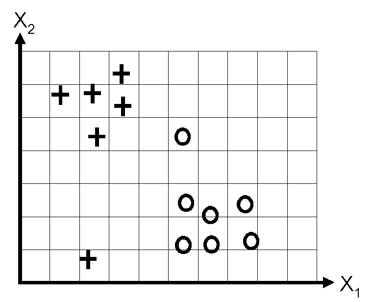
Suppose that we fit a logistic regression model with a bias weight \(w_0\), that is \(p(y \te 1\g \bx, \bw) = \sigma(w_0 + w_1 x_1 + w_2 x_2 )\), by maximum likelihood, obtaining parameters \(\hat{\bw}\). Sketch a possible decision boundary corresponding to \(\hat{\bw}\). Is your answer unique? How many classification errors does your method make on the training set?
Now suppose that we regularize only the \(w_0\) parameter, that is, we minimize \[ J_0(\bw) = -\ell(\bw) + \lambda w_0^2, \] where \(\ell\) is the log-likelihood of \(\bw\) (the log-probability of the labels given those parameters).
Suppose \(\lambda\) is a very large number, so we regularize \(w_0\) all the way to 0, but all other parameters are unregularized. Sketch a possible decision boundary. How many classification errors does your method make on the training set? Hint: consider the behaviour of simple linear regression, \(w_0 + w_1 x_1 + w_2 x_2\) when \(x_1 \te x_2 \te 0\).
Now suppose that we regularize only the \(w_1\) parameter, i.e., we minimize \[ J_1(\bw) = -\ell(\bw) + \lambda w_1^2, \] Again suppose \(\lambda\) is a very large number. Sketch a possible decision boundary. How many classification errors does your method make on the training set?
Now suppose that we regularize only the w2 parameter, i.e., we minimize \[ J_2(\bw) = -\ell(\bw) + \lambda w_2^2, \] Again suppose \(\lambda\) is a very large number. Sketch a possible decision boundary. How many classification errors does your method make on the training set?