Optimizing \(D_\mathrm{KL}(p(\bw\g\D)||q(\bw;\alpha))\) tends to be difficult. The cost function is an expectation under the complicated posterior distribution that we are trying to approximate, and we usually can’t evaluate it.
The Laplace approximation fitted a Gaussian distribution to a parameter posterior by matching a mode and the curvature of the log posterior at that mode. We saw that there are failure modes when the shape of the distribution at the mode is misleading about the over-all distribution.
Variational methods fit a target distribution, such as a parameter posterior, by defining an optimization problem. The ingredients are:
A family of possible distributions \(q(\bw; \alpha)\).
A variational cost function, which describes the discrepancy between \(q(\bw; \alpha)\) and the target distribution (for us, the parameter posterior).
The computational task is to optimize the variational parameters (here \(\alpha\)).1
For this course, the variational family will always be Gaussian: \[ q(\bw;\; \alpha\te\{\bm,V\}) = \N(\bw;\, \bm,\, V). \] So we fit the mean and covariance of the approximation to find the best match to the posterior according to our variational cost function. Although we won’t consider other cases, the variational family doesn’t have to be Gaussian. The variational distribution can be a discrete distribution if we have a posterior distribution over discrete variables.
The Kullback–Leiber divergence, usually just called the KL-divergence, is a common measure of the discrepancy between two distributions: \[ D_\mathrm{KL}(p||q) = \int p(\bz) \log \frac{p(\bz)}{q(\bz)}\;\mathrm{d}\bz. \] The KL-divergence is non-negative, \(D_\mathrm{KL}(p||q)\!\ge\!0\), and is only zero when the two distributions are identical.
The divergence doesn’t satisfy the formal criteria to be a distance, for example, it isn’t symmetric: \(D_\mathrm{KL}(p||q)\ne D_\mathrm{KL}(q||p)\).
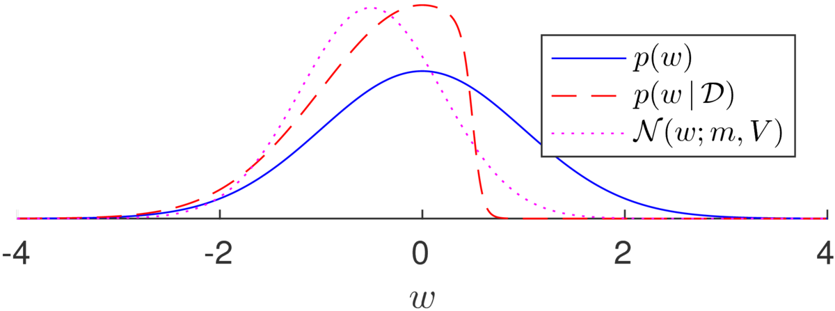
To minimize \(D_\mathrm{KL}(p||q)\) we set the variational parameters \(\bm\) and \(V\) to match the mean and covariance of the target distribution \(p\). The illustration below shows an example from the notes on Bayesian logistic regression. The Laplace approximation is poor on this example: the mode of the posterior is very close to the mode of the prior, and the curvature there is almost the same as well. The Laplace approximation will set the approximate posterior to be almost equal to the prior. While the posterior is clearly not a Gaussian, matching the mean and variance of the posterior is a better summary of where the plausible parameters are than the Laplace approximation:
Optimizing \(D_\mathrm{KL}(p(\bw\g\D)||q(\bw;\alpha))\) tends to be difficult. The cost function is an expectation under the complicated posterior distribution that we are trying to approximate, and we usually can’t evaluate it.
Even if we could find the mean and covariance of our distribution (approximating them would be possible) the answer may not be sensible. Matching the mean of a bimodal distribution will find an approximation centred on implausible parameters:
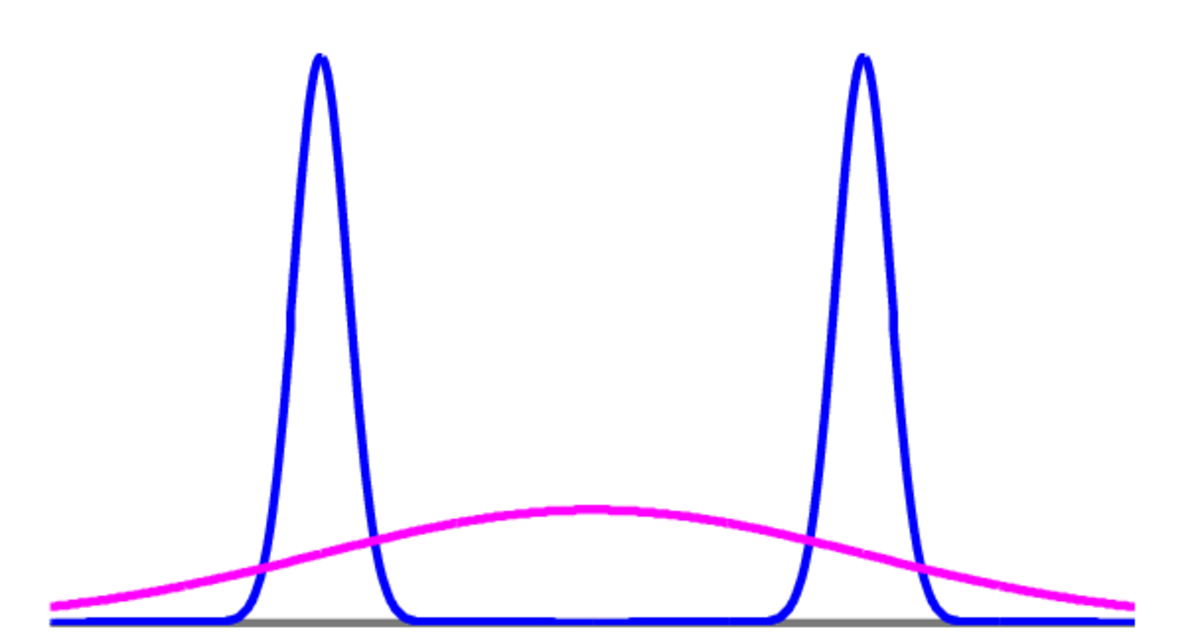
Our predictions are not likely to be sensible if we mainly use parameters that are not plausible given the data.
Most variational methods in Machine Learning minimize \(D_\mathrm{KL}(q(\bw;\alpha)||p(\bw\g\D))\), partly because we are better at optimizing this cost function. (There are also other sensible variational principles, but we won’t cover them in this course.) Minimizing the KL-divergence this way around encourages the fit to concentrate on plausible parameters: \[\begin{aligned} D_\mathrm{KL}(q(\bw;\alpha)||p(\bw\g\D)) &= \int q(\bw;\alpha) \log \frac{q(\bw;\alpha)}{p(\bw\g\D)}\;\mathrm{d}\bw\\ &= -\int q(\bw;\alpha) \log p(\bw\g\D)\;\mathrm{d}\bw +\underbrace{\int q(\bw;\alpha) \log q(\bw;\alpha)\;\mathrm{d}\bw}_{\text{neg.\ entropy,~}-H(q)} \end{aligned}\]
To make the first term small, we avoid putting probability mass on implausible parameters. As an extreme example, there is an infinite penalty for putting probability mass of \(q\) on a region of parameters that are impossible given the data. The second term is the negative entropy of the distribution \(q\).2 To make the second term small we want a high entropy distribution, one that is as spread out as possible.
Minimizing this KL-divergence usually results in a Gaussian approximation that finds one mode of the distribution, and spreads out to cover as much mass in that mode as possible. However, the distribution can’t spread out to cover low probability regions, or the first term would grow large. See Murphy Figure 21.1 for an illustration.
If we substitute the expression for the posterior from Bayes’ rule, \[ p(\bw\g\D) = \frac{p(\D\g\bw)\,p(\bw)}{p(\D)}, \] into the KL-divergence, we get a spray of terms: \[ D_\mathrm{KL}(q||p) = \underbrace{\mathbb{E}_q[\log q(\bw)] -\mathbb{E}_q[\log p(\D\g\bw)] -\mathbb{E}_q[\log p(\bw)]}_{J(q)} + \log p(\D). \]
The first three terms, equal to \(J(q)\) in Murphy, depend on the variational distribution (or its parameters), so we minimize these terms. The final term, \(\log p(\D)\) is the log-marginal likelihood (also known as the “model evidence”). Knowing that the KL-divergence is non-negative gives us a bound on the marginal likelihood: \[ D_\mathrm{KL}(q||p)\ge0 ~\Rightarrow~ \log p(\D)\ge -J(q). \] Thus, fitting the variational objective is optimizing a lower bound on the log marginal likelihood. Recently “the ELBO” or “Evidence Lower Bound” has become a popular name for \(-J(q)\).
The literature is full of clever (non-examinable) iterative ways to optimize \(D_\mathrm{KL}(q||p)\) for different models.
Could we use standard optimizers? The hardest term to evaluate is: \[ \mathbb{E}_q[\log P(\D\g\bw)] = \sum_{n=1}^N \mathbb{E}_q[\log P(y\nth\g\bx\nth,\bw)], \] which is a sum of (possibly simple) integrals. In the last few years variational inference has become dominated by stochastic gradient descent, which updates the variational parameters using unbiased approximations of the variational cost function and its gradients.
Reading for variational inference in Murphy: Sections 21.1–21.2.
Laplace approximation:
Variational methods:
The KL-divergence gives the average storage wasted by a compression system that encodes a file based on model \(q\) instead of the optimal distribution \(p\). MacKay’s book is the place to read about the links between machine learning and compression.
The textbooks often avoid parameterizing \(q\) in their presentations of variational methods. Instead they describe the optimization problem as being on the distribution \(q\) itself, using the calculus of variations. We don’t need such a general treatment in this course.↩
\(H\) is the standard symbol for entropy, and has nothing to do with a Hessian (also \(H\); sorry!).↩