|
To collect experimental evidence to support a hypothesis, we need to design and implement an experiment, and then analyse the results. We may need multiple passes to ensure that our experiment collects evidence capable of addressing our hypothesis. We may need to conduct exploratory data analysis in order to understand why our initial experiments are not meeting our needs and to help us adjust our experimental design accordingly. In these notes, we address these issues using an example experiment as a vehicle. The example and the analysis are based on a half-day tutorial by Paul Cohen, to whom I am grateful for his original slides and his helpful clarification of several issues.
These notes are divided into 5 'lessons':
As I already emphasised at length in The Need for Hypotheses in Informatics, the purpose of an evaluation is to confirm (or refute) a hypothesis or claim. It is thus essential that, when designing an evaluation, we must first clarify what claim it is supposed to test. Several claim templates are given here, followed by a discussion of the space of possible claims. Note that the best claims don't just state a property of or relationship between techniques, but they postulate a reason for that property or relationship: a 'because' clause. As we will see, such reasons will help in the design and analysis of experiments.
It is not enough merely to build a system and then ensure that it runs fine on some test data. That is testing, not evaluation. Testing is a (fallible) way to ensure that your program meets its specification. Scientific advance is only achieved when evaluation shows that a claim is true (or false).
Our worked example will be to compare two scheduling algorithms for a ring of processors. Each processor in the ring has two neighbours and a queue of jobs, which it completes in sequence.
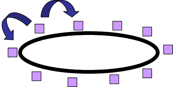
During processing, a job may divide into two new jobs. The processor will add one of these jobs to its own queue and give one to one of its neighbours. The two scheduling algorithms differ only in how they allocate the job they don't keep.
The process of job spawning can be envisaged as a binary tree, where each fork represents one job spawning two new ones. A theoretical investigation showed that KOSO* was superior to KOSO for balanced trees, i.e., when jobs spawning other jobs was controlled and balanced. However, the case of unbalanced trees resisted theoretical analysis. Cohen and his colleagues decided to design an experiment to compare KOSO and KOSO* for unbalanced trees. This arises when the probability of job spawning varies during a trial.
So, the first step is to make an explicit claim to be evaluated by this experiment. Superficially, KOSO* looks like a slightly more intelligent algorithm, but can we crystallise its superiority over KOSO?
Claim: KOSO takes longer than KOSO* because KOSO* balances loads better.
Note the 'because' phrase which gives a reason that KOSO* might be expected to take less time that KOSO. Load balancing is a critical property of parallel processing schedulers. It means that each processor gets a roughly equal load, say the same number of jobs waiting in their queues. The reason this is important is that if a processor runs out of jobs then it is idling while others are busy, which is a waste of processor time. It is crucial to keep all processors busy while jobs last.
In an experiment, there are always two kinds of variable: independent and dependent. The dependent variables are the results of the experiment: the ones you measure and analyse. The independent variables are the inputs to the experiment: the ones you vary to compare different conditions. The dependent variable in our experiment will be the total run time of all the jobs in a trial. The independent variables will be: whether KOSO or KOSO* was used for scheduling, the number of processors in the ring, the total number of jobs generated and the probability that a job will spawn. Recall that Cohen et al were interested in unbalanced trees, i.e., trials during which the probability of job spawning varies.
The initial results of Cohen's experiment were disappointing. After taking an average run time for KOSO and for KOSO* over several trials, the mean time for KOSO was 2825 and for KOSO* was 2935, i.e., KOSO was actually 4% faster than KOSO*, which is the opposite of our claim. Although the result turned out not to be statistically significant (see Lesson 5 for what this means), the result is nevertheless surprising. What happened?
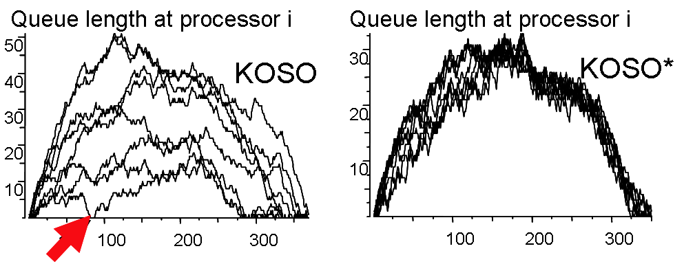
To find out what went wrong, we have to do some exploratory data analysis. There are various techniques we can use to help us visualise experiments. One common and useful technique is to construct time series. For each processor, we can plot queue length against time. The queue starts off empty, gets longer as new jobs are spawned and then decreases again as the jobs start to run out. We see that this does show evidence of better load balancing for KOSO*. At each moment of time, the KOSO* processors have roughly equal queues, whereas the KOSO ones vary widely in length. However, despite this varying queue length, we also notice that it rarely happens that a KOSO processor is starved of jobs, i.e., has an empty queue when their are jobs left to be done. We see one example where the red arrow points in the time series below. As long as KOSO processors have non-empty queues, they will not idle, so unbalanced loading will not result in slower overall speeds.
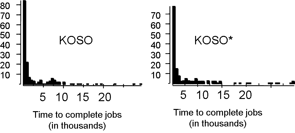
Another useful exploratory data analysis technique is to construct frequency distributions. This is a bar graph, with one bar for each time period. In our case the times will be the run times of jobs and the periods will cluster these into run times of similar length, e.g., intervals of a millisecond. The height of each bar indicates the frequency of events falling in that time period, e.g., the frequency of job run times in each period. In Cohen's experiment, most jobs took only a short time, so the highest bar corresponded to the period of shortest run times. The bars then decreased in height very quickly with periods of longer run time. There were a handful of outliers, i.e., rare events. That is, a very few jobs took a long time and were represented by short bars to the extreme right hand side of the graph.
In Cohen's experiment the results of several trials were averaged. This is a common analysis technique to avoid results being skewed by noise during a trial. The idea is that noise will be random across trials so will be lost in the averaging process. Several different kinds of averaging are possible: arithmetic mean, geometric mean, median, etc. Initially, Cohen used arithmetic mean, whereby all the results are summed and then divided by the number of trials. Unfortunately, means are overly influenced by outliers. Consider the following sequence of numbers: 1, 2, 3, 7, 7, 8, 14, 15, 17, 21, 22. The mean of these numbers is 10.6. However, if we add an outlier, say 1000, the mean jumps to 93.1. Medians, on the other hand, are quite robust against outliers. Without the outlier the median of the previous sequence is 8, whereas with the outlier it increases only to 11. The lesson is that where there are a handful of outliers, as with the KOSO vs KOSO* experiment, then we should use the median rather than the mean.
If we compare median total run times in the KOSO vs KOSO* experiment then KOSO's median is 498.5, whereas KOSO*'s is 447.0, i.e., KOSO* is 11% faster if we compare medians, but 4% slower if we compare means. While this is an improvement it is, unfortunately, still not statistically significant.
So, what is a median? Consider a graph in which the x-axis is ordered, for instance, a frequency distribution. Consider the area under that graph. With vertical lines we can divide that area into fragments. For instance, there is a vertical line that divides the area into two equal parts. The value of x at which that line crosses the x-axis is the median. More generally, we can divide the area into 100 equal parts with 99 such vertical lines. These lines are called quantiles. The 50th quantile gives the median; the 25th quantile gives the lower quartile and the 75th quantile gives the upper quartile. [NB -- note the difference between quantiles, with an 'n', and quartiles, with an 'r'.]
Now we have completed our exploratory data analysis, we need to use it to redesign our experiment. How shall we do that?
To see an advantage from the expected better load balancing of KOSO*, we'll have to arrange the independent variables to increase the chances of processor starvation. The easiest way to do this is to increase the number of processors until there is sometimes not enough jobs to go around. Cohen carried out the experiment again, but varying the number of processors in the ring between 3, 9, 10 and 20. This time there was significant processor starvation in KOSO experiment with 20 processors. Unfortunately, the results were still not statistically significant. Why not?
The problem is that variance in a problem can arise from any difference in the independent variables. In this case the only differences we actually care about are that between:
Unfortunately, differences caused by the other independent variables are much greater than those caused by the independent variables we care about. This makes it difficult to pick out the KOSO vs KOSO* signal from all the noise caused by other variance. In particular, statistical tests of significance demand a bigger observable difference to ensure that any effect is not caused by noise.
One solution to this problem is to increase the number of trials, systematically varying the independent variable settings, in the hope that the effect of other causes of variance will be cancelled out, leaving a clear signal from the variance we want to measure. However, the number of trials required will rise exponentially with the number of independent variables. This can make the experiment time-consuming and expensive. If there are many independent variables with many settings each, the number of trials could become astronomical. Moreover, when there are many different independent variables with many possible settings, a smarter solution is to redesign the dependent variable so that it controls for the unwanted variance. That solution is the topic of the next section.
We now see how to redesign the independent variable to control for unwanted variance. We perform a variance-reducing transform. To simplify the discussion, assume that each job takes unit time, then:
R is a new measure of run time restated to be independent of both number of jobs generated and the number of processors in the ring. By design it will be immune to any noise introduced by these two independent variables. Only differences due to either KOSO vs KOSO* or the probability of job spawning will show up in the experimental results. Note that the variance due to the probability of job spawning is deliberately not controlled for, because we are interested in investigating unbalanced trees.
We now run a series of trials. These can be envisaged using a cumulative distribution function, abbreviated as cdf. We plot the trial number on the x-axis and a running total of R on the y-axis, i.e., we add the R value for each trial to the running total so far. If we plot cdfs for KOSO and KOSO* for our experiment we will see the initial two graphs are almost indistinguishable, but as trials accumulate the KOSO cdf can be seen to rise quicker than the KOSO* cdf, which is what we hoped to see.

To check whether our experimental results are now significant, we need to perform a statistical test. In particular, we can average the values of R over several trials and then see whether the difference in the averages are statistically significant. For averaging we could use the arithmetic mean, the median or some other measure. The following table shows the results for both mean and median.
| Mean | Median | |
| KOSO | 1.61 | 1.18 |
| KOSO* | 1.40 | 1.03 |
The ideal result here is 1, which would indicate perfect parallelism. From the table we can see that the median of KOSO* is 1.03, which is very close to such perfection. Also, for both the mean and the median, the averages for KOSO* are closer to 1 than are those for KOSO. This looks quite promsing, but to be sure it is statistically significant, and not just a result of noise from unwanted variance, we need to perform a statistical test
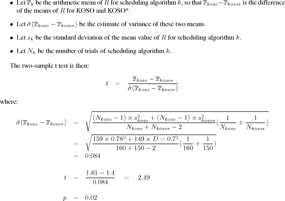
The statistical test chosen by Cohen et al was the two-sample t test. This is a popular test, which is relatively simple to understand and apply. It does have the drawback that it works on means rather than medians - and we argued above that medians were a better measure - but we'll live with that.
The function t is defined as the difference between the two means divided by an estimate of the variance of the difference between these two means. The greater the difference between the means, then the greater t will be. In our example this difference is 1.61-1.40=0.21. However, this is tempered by the variance estimate. The larger this variance is then the smaller t will be. In our example this variance estimate will turn out to be 0.084. We can now calculate t=0.21/0.084=2.49. There is a standard way to convert values of t into probabilities. In our case t=2.49 converts into p=0.02. This probability gives the likelihood that there is no difference in the performance of KOSO and KOSO*: the, so called, null hypothesis. The probability 0.02 is our residual uncertainty that we might be wrong. Each scientific field has developed a threshold below which a residual uncertainty can be ignored and the hypothesis considered to be confirmed. For experiments on computer systems, a figure of 0.02 is well below this threshold. So the null hypothesis is very unlikely to be true, meaning that the observed difference in average run time between KOSO and KOSO* is statistically significant. At last we have an experimental result that confirms our hypothesis.
This t-test formula reflects our aims in the experimental design. On the one hand, the greater the difference between the run times of KOSO and KOSO* then the more confident we will be in our result. On the other hand, we need to minimise the unwanted variance to be sure that this difference reflects a difference in performance of KOSO and KOSO*, and is not due to some other cause.
To calculate the variance of the difference we need the means, their standard deviations and the numbers of trials of KOSO and KOSO*. The standard deviation is a measure of the variation from the mean. A low standard deviation indicates that the data points tend to be very close to the mean, whereas high standard deviation indicates that the data is spread out over a large range of values. The values of these measures for our example are given in the following table.
| Mean | Standard Deviation | Number of Trials | |
| KOSO | 1.61 | 0.78 | 160 |
| KOSO* | 1.40 | 0.7 | 150 |
The calculation of t is now as follows:
It's worth reiterating the logic of statistical tests, as it can be initially confusing and unintuitive.
We can summarise the experimental methodology as follows.
|
Informatics Forum, 10 Crichton Street, Edinburgh, EH8 9AB, Scotland, UK
Tel: +44 131 651 5661, Fax: +44 131 651 1426, E-mail: school-office@inf.ed.ac.uk Please contact our webadmin with any comments or corrections. Logging and Cookies Unless explicitly stated otherwise, all material is copyright © The University of Edinburgh |

