Before we look more closely at some of the in-principle problems with massive PCFGs

• Such as we get in the case of built-from-treebanks grammars

We'll look at some practical difficulties

Multiple tags per terminal (word)

• Plus 100s, if not 1000s, of rules for some non-terminals (categories)

Means 100s of thousands of edges in a probabilistic chart parser

If we're working with spoken language, the numbers are even worse

• As there will be multiple alternative hypotheses about the words in the utterance
• "people can easily recognise speech"
• "people can easily wreck a nice beach"

Finding all the parse trees, so that you are sure to find the best, is often therefore out of the question

• Charniak reports, for instance, that getting 95% of the way to finding all parses
• Of a 30-word sentence from the Brown corpus
• With a PCFG constructed from the Brown corpus
• Took 130,000 edges

More recent experiments

• with highly optimised representations of the parse trees
• required 24 gigabytes of storage to hold complete sets of parses

So although what I said yesterday is true in principle

• That is, that maintaining an ordered edge queue makes a chart parser best-first
• In practice the cost of doing so is very high
  • Prohibitively high for broad-coverage probabilistic grammars
• Because it turns into breadth-first search across all possible parses constructed left-to-right

Why is this?

• In the first instance, because of the product of probabilities problem

. . . produces small numbers quickly

So short analyses are almost always are more probable than long ones

• And shallow ones are more probable than deep ones

Consider the trivial case of the three word phrase "the men "

• Here are the MLE estimates of eight relevant probabilities
  • Taken from NLTK

• DT → 'the'  0.49455
• JJ → 'the'  0.0008570
• NNS → 'men'  0.001653
• NP-SBJ → DT NNS  0.017011
• NP-SBJ → JJ NNS  0.010468
• VBD → 'came'  0.006901
• VP → VBD  0.002619
• S → NP-SBJ VP  0.39202

And here are the costs (that is $-{\log }_2\left(\text{prob}\right)$)

• DT → 'the'  1.02
• JJ → 'the'  10.19
• NNS → 'men'  9.24
• NP-SBJ → DT NNS  5.88
• NP-SBJ → JJ NNS  6.58
• VBD → 'came'  7.18
• VP → VBD  8.58
• S → NP-SBJ VP  1.35

It turns out that even though analysing 'the' as DT is 500 times more likely than analysing it as JJ

• We'll still keep taking both analyses forward through a best-first parse to the very end

Here are the two key subtrees, with their accumulated costs:

Even though the 'wrong' NP-SBJ has much higher cost that the 'right' one

• the extra consitutent cost for the whole 'right' sentence is even higher
• so the 'wrong' NP-SBJ will be added to the chart before the 'right' S
• and quite possibly before many other 'wrong' partial analyses based on it

What we've been using to order the agenda is called the inside probability

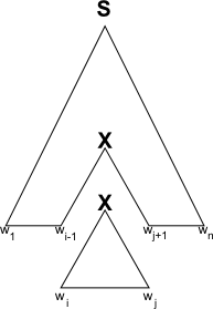
• In practice, the inside cost

• That is, the probability for some node X that it expands to cover what it covers
• $P(\mathrm{NT}\to *w_{\mathrm{i}}...w_j|\mathrm{NT})$
• It's also helpful to define the notion of outside probability:
  • The probability that the rest of the tree is what it is
  • $P(S\to *w_1...w_{\mathrm{i-1}}X{w}_{\mathrm{j+1}}...w_n)$

Using the inner probability to sort the agenda will clearly prefer smaller trees

• We need to introduce some kind of normalisation to avoid this
• Understanding as we do so that we may thereby put at risk our goal of getting the best parse first

The name for what we're looking for is a figure of merit

• That is, some non-decreasing measure of (partial) subtree cost

There are lots of possibilities

• Of which most obvious is also the simplest
• Inner cost, normalised by word span

This would clearly have the desired effect in our worked example above

• The cost of the first inactive NP-SBJ edge is divided in half
  • From 16.14 to 8.07
  • Thereby ensuring that it will be processed before the implausible 'the'-as-adjective hypothesis

Note that normalising in the cost domain uses the arithmetic mean

• because we've been summing costs

In the probability domain, we use the geometric mean

• because we've been multiplying probabilities

Using the left half of the outer cost as well improves performance further

• In principle
• But in practice takes too much time to compute

See Caraballo and Charniak 1996 for the details

Even with a good figure of merit, our chart will still grow very large

• If we pursue every hypothesis, no matter how expensive

So standard practice is to prune the agenda

• That is, set a maximum number of edges we will hold
• Or a maximum delta between the best and worst that we will hold

The result is called beam search

• And the relevant parameter the beam width

Whenever the agenda is full

• that is, has the number of entries specified by the beam width
• and we need to insert an edge

There are two possibilities (ignoring ties)

• If the new edge is more expensive than the most expensive edge in the agenda
  • We discard the new edge
• Otherwise we discard the current most expensive edge
  • and insert the new edge at its appropriate place in the agenda