Answers and Explanations for Lab 2
| Author: | Sharon Goldwater |
|---|---|
| Date: | 2014-09-01 |
| Copyright: | This work is licensed under a Creative Commons Attribution-NonCommercial 4.0 International License: You may re-use, redistribute, or modify this work for non-commercial purposes provided you retain attribution to any previous author(s). |
Examining and running the code
If you type this into the interpreter:
%run lab2.py
You will get an error message You must provide at least one filename argument. (This is followed by a further, completely generic, error message simply saying that an exception has occurred, i.e., the program has exited unexpectedly.) The error message is generated by a print statement in the main body of code (near the end of the file), which gets called if sys.argv is less than 2 (i.e., no arguments are provided).
fnames is a list which stores the names of the files that are to be processed.
word_counts is a dictionary (or to be precise, a defaultdict), whose keys are the words and values are their counts.
In the first two Ethan files, 'the' occurs 268 times, which you can see by typing word_counts['the'] in the interpreter.
Looking at the data
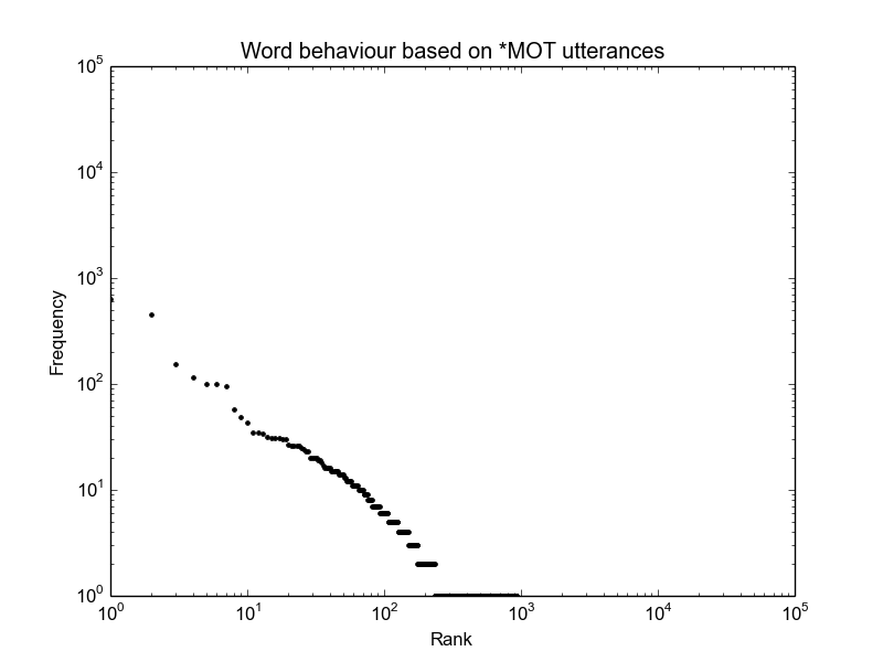
The Zipf plot from eth01.cha is shown below. The main problem that can be seen (if you know what to look for, and you must look at the log-log plot) is that there are too many words with frequency one, which shows up as a very long horizontal line at the bottom. It is maybe not completely obvious from this plot, but if you generate the plot from all the Ethan files together, it becomes much more obvious.
- How many unique word types are there?
len(word_counts)
In this particular case, it probably won't be obvious how many unique word types there ought to be, so doing this won't help much initially, but it's useful for helping to verify later that you have fixed the problem.
- What are the first few and last few words as sorted alphabetically?
sorted(word_counts.keys())[:10]
sorted(word_counts.keys())[-10:]
These lines will give you the first 10 and last 10 words. The last 10 look fine, but the first 10 do not look like real words, instead they look like \x151000080_1006955\x15. This indicates the first problem -- we have included the timestamp IDs in the word counts, which we should not have done.
- What are the first few and last few words as sorted by frequency?
sorted(word_counts, key=word_counts.get)[:10]
sorted(word_counts, key=word_counts.get)[-10:]
The 10 lowest frequency words (first line above) are the same junk words we got by looking at the alphabetical sort, which makes sense because each of these only occurs once (the timestamps are unique). The 10 highest frequency words (second line above) include some actual high-frequency words like 'your' and 'the', but also some punctuation marks and the token *MOT (which is actually the highest frequency item). The latter is definitely a problem, since it isn't a word but instead identifies who is speaking. The punctuation marks may or may not be a problem depending on how we want to define a word and what we might be doing with the data.
- Modify the zipf_plot function so that the words themselves show up as the x-axis labels.
See our answer code.
Fixing the problem
You can take a look at our very simple solution in the answer code. It simply strips off the first token (the speaker ID) and last two tokens (final punctuation mark and timestamp ID) before adding the tokens to the word_counts dictionary. The decision to strip off final punctuation is maybe a bit inconsistent because we still have internal punctuation (commas etc) in the counts; we could have chosen to leave the final punctuation on.
Other possible non-words include sound effects ('boom', 'boo', 'ah', etc) and alternate spellings ('(a)bout'), as well as punctuation.
When you run the code on all the files, it looks smoother because the statistics of large data sets become closer to 'average' -- the randomness of small sample sizes begins to smooth out.
MLU
- What do the variables ntoks and nutts represent? Can you explain the line where ntoks gets incremented and why there is a -3 there?
These variables represent the running total number of word tokens and number of utterances in each file. To compute the MLU for a file, we need to divide ntoks by nutts. For each line (utterance) spoken by the child, ntoks is incremented by the the number of (whitespace-separated) words in the line (computed as len(tokens)) minus 3. We subtract 3 because we do not want to include the speaker ID, final punctuation, or timestamp ID in the count of words spoken by the child. (We would get a more accurate MLU by also throwing away other punctuation inside the sentence, but we are trying to keep things simple here and we'll still have a reasonable approximation.)
- Complete the code to create MLU plots.
See answer code for our solution.
- What general trends do you see in the plots and why? Why are the plots so jagged?
In general, you should see that the children's MLUs increase over time, starting at around 1-1.5 and going up to 3.5 or more in most cases. There are a lot of ups and downs in the plots because each of the files is a fairly small sample of language, so there will be quite a bit of random variation in the MLU.
- Suppose we wanted to use this data to directly compare the language development of the different children, i.e., whether one child is acquiring language faster than another. What information is missing from the plots you just made that would be needed in order to do this analysis?
The key additional piece of information we would need is the actual ages of the children. For example, if we look at the plots, it appears that Alex's language is hardly developing at all, whereas Naima's MLU is around 5 by the end of the data. However, from these plots alone we do not know whether the time range spanned by the Alex files is the same as that of the Naima files. We would want to know both whether the files start at the same ages for each child, and also whether the period of time between each file is the same.